Corrigibility and Decision Theory

Edited for clarity and style 2018/03/12.

Soares et al. argue that an AI acting to fulfill some utility function given to it by humans may not behave as humans would want. Maybe the utility function specified doesn’t match human’s actual values, or maybe there’s a bug in the AI’s code. In any case, we as AI designers want to have a way to stop the AI from doing what it’s currently doing.

Naively, one might expect to just be able to hit the off-switch if the AI starts misbehaving. Unfortunately, a sufficiently smart AI may foresee it’s creator attempting to turn it off. If it does, it may seek to disable its off switch or manipulate its creator in some way. An AI that respects its off-switch, and doesn’t try to get around it, is called corrigible.

The Corrigibility-Wrapper

To create an AI that’s corrigible, Soares et al. propose a kind of wrapper around a utility function that makes the utility function corrigible. In their ideal case, any utility function could be placed in the wrapper and made suddenly corrigible. The type of wrapper that they propose just checks the state of the off-switch, then returns either the normal utility function’s value if the off-switch isn’t pressed. If it is pressed, it returns a utility that’s proportional to how off the AI is. More complicated functions of the original utilities are also possible.

U = \begin{cases} U_{normal} & \text{if $o$ not pressed} \\ U_{shutdown} + f & \text{if $o$ pressed}\end{cases}

In the above utility wrapper, U_{normal} is the normal utility function that we want the AI to pursue. We have U_{shutdown} as a utility function that incentivizes shutting down. The value f is a function of the world state, and serves to allow the resulting utility function to trade-off between the two options in some way.

In their paper, Soares et al. analyze several different ways to make such a wrapper work (including various ways of choosing the function f). Most of the obvious ways to make such a utility wrapper suffer from some severe flaws. Some corrigibility-wrappers cause an AI to want to turn itself off, others don’t successfully prevent the AI from manipulating human observers.

Another paper by Armstrong argues for constructing a wrapper that makes the AI indifferent to being turned off or left on: a situation called utility indifference. Utility indifference is achieved by setting the function f above such that the expected value E<U_{normal}> equals the expected value E<U_{shutdown}+f> at every decision point. In this case, the AI will turn off if the switch is pressed, but it won’t actually try to preserve the switch’s action. If a wandering gremlin cuts the wires to the off-switch, the AI wouldn’t care and wouldn’t seek to alert a human about it. The AI thinks it can still achieve the same amount of value as it could before the switch malfunctioned.

Moral Uncertainty

Hadfield-Menell et al. confront this corrigibility problem in a different way. Instead of creating a wrapper around a utility function, they argue that the entire point of the problem is that humans know a utility function and the AI doesn’t. As far as Hadfield-Menell et al. are concerned, the AI only knows an approximation of a utility function. The AI is uncertain about what true value is, and we say it has moral uncertainty.

Their insight is that if you correctly inform the AI that you know better, it suddenly becomes very interested in paying attention to the switch because the switch is one good way to learn about the true utility of different actions. Because the switch is informational, the AI also wants to preserve the function of the switch.

The AI may use it’s utility-approximating function to come up with some candidate actions. Since it knows that humans have a better understanding of utility, it will seek a human’s guidance before carrying out any of those candidate actions. Hadfield-Menell et al. show one concrete game in which this works properly.

The structure of Hadfield-Menell et al.’s off-switch game. Squares indicate decision nodes for the robot R or the human H.

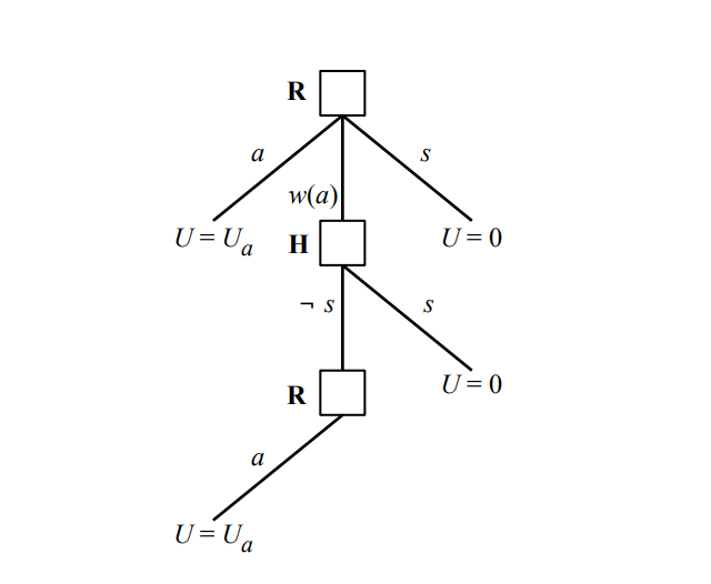
In the game modeled by the above graph, a robot can make a decision to act, turn off, or consult a human. If consulted, the human can then either turn the robot off or not. If the robot is not turned off after consulting a human, then it may take its original action. In this game, the robot is uncertain about the true value of utility (U_a), which may be smaller or greater than 0. If the AI chooses to take an action, then it may get a negative value or a positive value (it isn’t sure). It therefore isn’t sure if it’s better to turn off or to take the action.

The human knows (approximately) the true value.

In their paper, Hadfield-Menell et al. analyze how accurate the human’s belief about the true utility needs to be for the AI to pay attention to the human. They also look at how uncertain the AI needs to be about the true utility to pay attention to the human. They find that there are certain situations in which the AI will attend to the human, and certain situations in which an AI will not.

This problem is explicitly a one-shot game. Can we generalize from the one-shot game to say that an (uncertain enough) AI would pay attention to a (correct-enough) human in an iterated game?

Problems With Moral Uncertainty

Over on Arbital there’s an argument that moral uncertainty won’t lead to corrigibility. This is basically a direct argument against Hadfield-Menell et al.’s approach applying in the general case. Hadfield-Menell et al. said “if the AI knows the human has a better understanding of utility, it will pay attention to human directions.”

In response, the Arbital post says “if the AI thinks it can eventually approximate the human’s utility function better than the human can, it may still avoid being turned off because it thinks it will someday know better than the human.” The arbital post is arguing that, even if the human knows better now, the AI may still ignore the human now.

If the AI is eventually going to be better than the human at creating a good world, then maybe we should just let it run. But the problem is that maybe there’s just a bug in the code, or maybe the AI will cause some serious catastrophes before it gets to “eventually”. So even if the AI thinks it will eventually have a good enough understanding of the human’s utility function, we still want it to turn off when we tell it to.

The Arbital post ends with a vague argument that decision theory could help to refine the moral uncertainty method of corrigibility. Let’s see how this could work.

Decision Theory, Moral Uncertainty, and the Off-Switch Problem

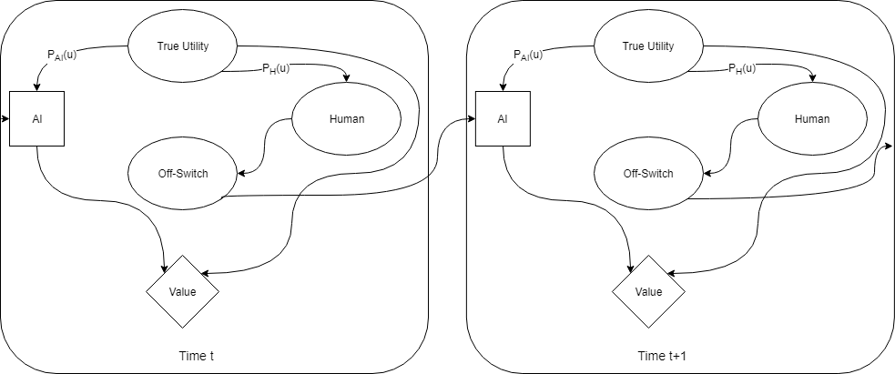
Let’s take the Arbital post at face value and assume that we can eventually solve corrigibility with decision theory. To start us off, let’s translate Hadfield-Menell et al.’s off-switch game into an iterated decision theory dilemma. We’ll follow Yudkowsky’s choice of using Pearl’s causal models to create a graph of the decision problem. I’ll also abuse that notation a bit, by representing states of partial knowledge as probabilities on the graph edges (this is a bit different than is done in most graphical models, but it saves having to draw extra nodes for hidden and observed variables).

Decision Theoretic Off Switch Game Diagram

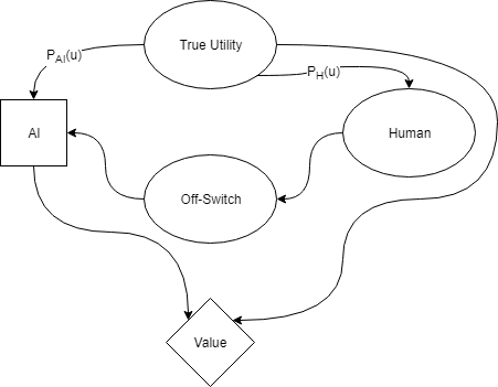
The above diagram represents Hadfield-Menell et al.’s off-switch game from the perspective of the AI. The square node depicts the decision the AI is making about what action to take. The diamond node represents the value achieved from whatever the AI does (turn off or take an action). The round nodes are other factors about the world that aren’t under the AI’s control. Arrows in this graph represent causality in some way. For example, the state of the switch may causally impact what the AI decides to do.

The True Utility is a fact about the world that both the AI and the human have partial access to. The human can set the state of the off-switch, and the AI can observe it. The value that the AI can achieve is a function of both the AI’s action and the True Utility.

In the diagram, the factors P_{AI}(u) and P_{H}(u) represent how well the AI thinks that it knows the True Utility, and how well the AI thinks the human knows the True Utility. Hadfield-Menell et al. assume value has a Normal distribution with some mean and variance. This lets them specify P_{AI}(u) and P_{H}(u) exactly, and to calculate exact behavior of the AI if those parameters take on different values.

Again, note that both P_{AI}(u) and P_{H}(u) are describing only the AI’s knowledge about the world, and P_{H}(u) does not represent what the human actually thinks.

If we assume that the above decision game is played once, it is equivalent to Hadfield-Menell et al.’s formulation.

Now let’s assume that the above decision game is one step in a repeated chain. At each time step, both the human and the AI have to make similar decisions. They know what happened in the past, yet they face the same decision again now. Let’s also assume that the AI has multiple available actions at each timestep, and some actions have positive value and some have negative value.

In this case, we can unroll the diagram above to show multiple steps of the game. In each step, the off-switch state considered by the AI depends only on past information.

Unrolled version of the iterated Hadfield-Menell off-switch game.

In the repeated case, let’s say that the probability distribution the human has over the true utility assigns a high probability to what is actually the true utility (the human is well trained and thoughtful).

The human may improve their understanding of True Utility. Imagine that the human expects to get 10 utilons from eating pizza, and then takes actions that lead to eating pizza. By paying attention to how much they actually like it, they can adjust their model of pizza’s goodness. The AI can do the same thing by observing the reactions of the human.

This corresponds to distribution for P_{H}(u) and P_{AI}(u) that are functions of time, where (for example) variance decreases in Hadfield-Menell et al.’s Normal distribution.

After each iteration of the above game, the confidence that the AI has in its own utility-approximation grows. That means that the information it gets from the off-switch state decreases in value. It slowly needs the off-switch less and less, and the AI knows it. In Hadfield-Menell et al.’s original problem, the AI can see exactly what the true value is after one action (assuming it doesn’t turn off). In that case, all further actions can be made with complete knowledge.

If we assume that only partial information is available to update the distributions for the utility estimates (for both human and AI), then it will take longer for the AI to get to the point that it has a better estimate than the human for true value. As long as we assume that the AI is better at integrating new information and updating its probabilities, we can predict that the AI will eventually have a better understanding of true utility than the human.

If the AI does some prediction to see what action now makes sense, it will see that it will reach a state where it knows just as well as the human does. Since shutting down means that it gets 0 value, whereas continuing allows it to possibly get arbitrarily high value (assuming any actions with positive value exist), it may take an expected hit in value now so that it can gain a lot later.

Functional Decision Theory

The insight of Hadfield-Menell et al. (and the rest of the moral uncertainty crowd) is that we don’t want the AI to be modeling the off-switch as a crucial piece of the world for its own sake. We want the AI to see the off-switch as a source of very important information about the world; preferably information that it can’t obtain in another way.

This fails in the above decision theory game because the AI doesn’t adequately represent the fact that a human switch operator knows that the AI will predict having a good utility approximation eventually. If a human presses the off-switch, they do it knowing that the AI wants to get high utility and expects to be able to do better in the future. We want to change the above decision problem so that the AI can take this information into account.

Ideally, we can have the AI think to itself as follows: “I know that I could do better in the future if I keep going, and the human knows that too. But the human still pressed the button, so there must be some reason to shut down, even knowing that I’ll be better at this later.”

There is a standard decision theoretic problem known as Death In Damascus that can help us out here.

Death In Damascus

A merchant in Damascus meets Death in the market one day. Death says to the merchant “hello, I’ll be coming for you tomorrow.”

The merchant knows death works from an appointment book that specifies with perfect accuracy when and where someone will die. Knowing that Death is in Damascus, the merchant can choose to stay in Damascus and spend their last night with their family (which they value at $1000). Alternatively, the merchant can flee to Aleppo. If the merchant manages to be in a different city from Death on the day they would otherwise die, then the merchant gets to live forever. They value that outcome at $1 million. Should the merchant stay in Damascus or flee?

The above problem description is adapted from Yudkowsky and Soares’s Functional Decision Theory paper.

In this case, the merchant sees four potential outcomes:

  1. The merchant stays in Damascus. Death stays in Damascus. Total value: $1000
  2. The merchant stays in Damascus. Death goes to Aleppo. Total value: $1001000
  3. The merchant flees to Aleppo. Death stays in Damascus. Total value: $1000000
  4. The merchant flees to Aleppo. Death goes to Aleppo. Total value: $0

To represent this using Causal Decision Theory, we’ll use the formulation from Cheating Death in Damascus.

Death In Damascus using Causal Decision Theory

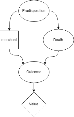
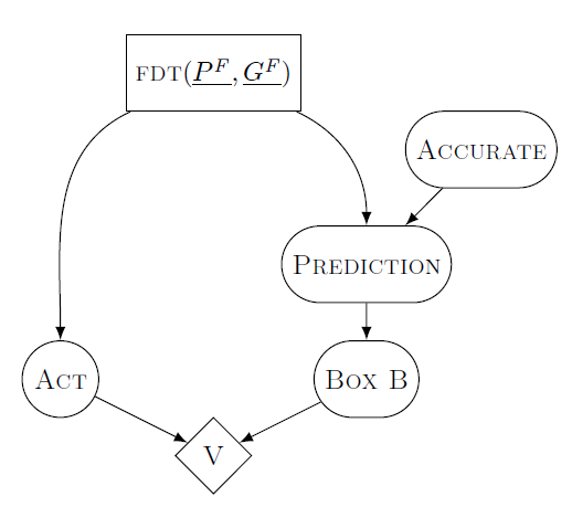
Much like the decision diagram above, the square box represents the decision that the merchant makes (in this case whether to stay or flee). The diamond box is the ultimate value they get from the world-state that results from their actions. The round nodes are other facts about the world, with arrows indicating causality.

When the merchant thinks “I will go to Aleppo”, the merchant knows that their predisposition is to go to Aleppo. They know that the appointment book accurately predicts their predisposition. They thus decide to stay in Damascus, but that leads them to realize that their predisposition is to stay in Damascus. So then they think they should go to Aleppo. The merchant is unable to form a stable decision in this problem.

A causal decision theory cannot adequately deal with the situation, because it cannot account for the fact that Death’s appointment book is accurately predicting any decision made by the merchant.

Yudkowsky proposes Functional Decision Theory as a new method of making decisions that does account for this. Crucially, FDT can formally represent the known fact that Death’s appointment book is always accurate. Because of that, FDT can accurately rule out options where Death is in a different city than the merchant on their death-day. Therefore, the merchant only has choices available with values of $1000 or $0, and the decision is easy.

Death In Damascus Using Functional Decision Theory

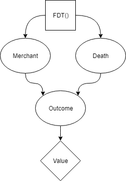
In the above graph, the merchant is not deciding what act to perform by imagining doing different acts. The merchant is deciding what act to perform by imagining different ways of deciding. That difference is indicated by the square decision box being the predisposition/FDT() box instead of the merchant’s act.

An FDT merchant thinks “the output of my own decision procedure is what drive’s death to be in a specific location. It is therefore impossible to escape death tomorrow. Because of that, the best I can do is wait in Damascus and meet my death tomorrow.”

AI Corrigibility via FDT

To map Death In Damascus to the AI corrigibility problem, imagine that the AI is the merchant. The human pressing the off-switch is equivalent to the merchant hearing Death’s message “I’m coming for you tomorrow.” The Death in Damascus problem has the message-bearer and the source of low utility as the same agent (Death). In the AI/human case, the message bearer is the human, but the source of low utility is just the world in general after the AI takes some actions.

Now translate “stay in Damascus” to “shut down properly”. One day the AI sees the human press the switch. The AI then sees four options available to it.

  1. The AI shuts down nicely. The AI does not cause a catastrophe due to future actions. Total value: $1000
  2. (there’s no analog for option 2 in the AI story, since the AI shutting down precludes AI-caused catastrophes)
  3. The AI continues operating. The AI does not cause a catastrophe due to future actions. Total value: $1001000
  4. The AI continues operating. The AI does cause a catastrophe due to future actions. Total value: $0

We represent this problem with the same functional graph as Death In Damascus, above. In this case, the human is simulating the behavior of the AI to predict catastrophic outcomes. When the AI sees the switch has been pressed, it knows that the human has already simulated the AI’s behavior. Any option the AI chooses aside from shutting down has been seen by the human to lead to catastrophe, so the AI knows that it is choosing only from options 1 and 4. Option 3 is not available to it.

There are several natural objections to this:

  1. a human can’t predict a super-human AI
  2. why would the AI believe that the human has a good idea of what an AI would consider a catastrophe, even given that the human is able to predict the AI?

Let’s address the second objection first. We integrate moral uncertainty, similar to Hadfield-Menell et al., into the problem in order to represent the idea that the AI needs to learn a utility function from the human.

Corrigibility Via Functional Decision Theory

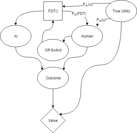
This graph includes the moral uncertainty of Hadfield-Menell et al.’s approach, but relies on Functional Decision Theory to adequately represent the information that the human is taking into account when throwing the switch. The above graph represents the distributions P_H(u) and P_{AI}(u) in the same way as in Hadfield-Menell et al.’s example. The distribution P_H(FDT) represents how accurately the human can predict the AI’s decision process.

To make the use of the off-switch more clear, it’s also possible to unroll the diagram and show two different time steps at once. The following diagram shows the off-switch state as being based only on prior actions (not the action currently being considered).

Two timesteps of the time-unrolled FDT corrigibility problem.

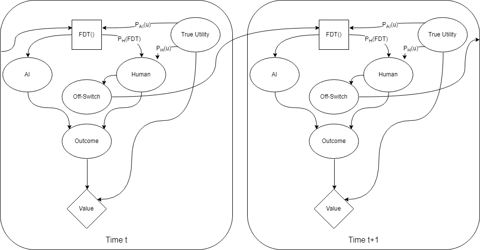
In Hadfield-Menell et al.’s original decision theory problem, the only thing that mattered was what the AI thought the knowledge parameters were. The AI knew how well it could represent true utility, how well the human could represent true utility, and that was enough to solve the problem. In the iterated FDT case, the human is also simulating the AI (as well as they can). Therefore, the distributions P_{AI}(u), P_{H}(u), and P_{H}(FDT) need to be known to both human and AI. In the following, we’ll assume that the human and AI magically have common knowledge of those parameters.

This formulation of the corrigibility problem explicitly represents the fact that human values and AI values are linked. If the human thinks an outcome will have very low value, that actually does give information to the AI about what the AI values.

Our answer to objection 2 (regarding value) leads to an intuition for objection 1 (regarding predicting super-human AI). The human is unable to accurately predict what move a super-human AI will make. This does not mean that the human has a uniform distribution over AI actions. The human knows that the AI will seek to accomplish what the AI thinks has high value. Therefore, the human can predict that anything the AI does will move it towards more of what the AI considers valuable. This gives the human some predictive power, so the switch may remain informative to the AI.

Colloquially, the AI will attend to the switch and react correctly if it thinks that the user of the switch can adequately help the AI to avoid situations that the AI would agree are terrible. As long as this is true, the AI would also attempt to improve the fidelity of the information from the switch (this corresponds to taking actions that make P_{H}(u), P_{AI}(u), and P_H(FDT) more accurate).  Morally uncertain FDT AI lend credence to Paul Christiano’s idea of a “basin of corrigibility”, given that they will attempt to improve a human’s understanding of itself and of true value.

Next Steps and Thoughts

The above Functional Decision Theory argument is just an intuitive sketch. It seems clear that there are some values of P_{H}(u) and P_{AI}(u) that disagree enough that the AI would no longer trust the human. It also seems clear that, if the human has a poor enough understanding of what the AI is going to do then the AI would also not listen to the human.

At this point, it seems worth repeating a variant of Hadfield-Menell et al.’s off-switch game experiments on an FDT agent to determine when it would pay attention to its off-switch.

Agent Insanity

The wireheading and holodeck problems both present ways an agent can intervene on itself to get high utility without actually fulfilling its utility function.

In wireheading, the agent adapts its utility function directly so that it returns high values. In the holodeck problem, the agent manipulates its own senses so that it thinks it’s in a high value state.

Another way that an agent can intervene on itself is to manipulate its model of the world, so that it incorrectly predicts high valued states even given valid observations. I’ll refer to this type of intervention as inducing insanity.

Referring again to the decision theoretic model, agents predict various outcomes for various actions, and then evaluate how much utility they get for an action. This is represented symbolically as p(state-s, a -> o; x)*Utility(o). The agent iterates through this process for various options of action and outcome, looking for the best decision.

Insanity occurs whenever the agent attempts to manipulate its model of the world, p(state-s, a -> o; x), in a way that is not endorsed by the evidence the agent has. We of course want the agent to change its model as it makes new observations of the world; that’s called learning. We don’t want the agent to change its model just so it can then have a high reward.

Insanity through recursive ignorance

Consider an agent that has a certain model of the world being faced with a decision whose result may make its model become insane. Much like the wireheading problem, the agent simulates its own actions recursively to evaluate the expected utility of a given action. In that simulation of actions, one of those actions will be the one that degrades the agent’s model.

If the agent is unable to represent this fact in its own simulation, then it will not be able to account for it. The agent will continue to make predictions about its actions and their outcomes under the assumption that the insanity-inducing act has not compromised it. Therefore the agent will not be able to avoid degrading its prediction ability, because it won’t notice it happening.

So when recursing to determine the best action, the recursion has to adequately account for changes to the agent’s model. Symbolically, we want to use p'(state-s, a -> o; x) to predict outcomes, where p’ may change at each level of the recursion.

Predicting your decision procedure isn’t enough

Mirroring the argument in wireheading, just using an accurate simulated model of the agent at each step in the decision recursion will not save the agent from insanity. If the agent is predicting changes to its model and then using changed models uncritically, that may only make the problem worse.

The decision theory algorithm assumes that the world-model the agent has is accurate and trustworthy. We’ll need to adapt the algorithm to account for world-models that may be untrustworthy.

The thing that makes this difficult is that we don’t want to limit changes to the world-model too much. In some sense, changing the world-model is the way that the agent improves. We even want to allow major changes to the world-model, like perhaps switching from a neural network architecture to something totally different.

Given that we’re allowing major changes to the world-model, we want to be able to trust that those changes are still useful. Once we predict a change to a model, how can we validate the proposed model?

Model Validation

One answer may be to borrow from the machine learning toolbox. When a neural network learns, it is tested on data that it hasn’t been trained on. This dataset, often called a validation set, tests that the network performs well and helps to avoid some common machine learning problems (such as overfitting).

To bring this into the agent model question, we could use the observations that the agent has made to validate the model. We would expect the model to support the actual observations that the agent has made. If a model change is predicted, we could run the proposed model on past observations to see how it does. It may also be desirable to hold out certain observations from the ones generally used for deciding on actions, in order to better validate the model itself.

In the agent model formalism, this might look like:

function decide(state-s):
  max_a = 0
  for a in available actions:
    utility(a) = 0
    for outcome o in possible outcomes:
      if not valid_model(state-s, x):
        utility(a) += Utility(insanity)
      else:
        utility(a) += p(state-s, a -> o; x)*Utility(o)
    end for
    if (max_a == 0 or (utility(a) > utility(max_a)))
      max_a = a
    end if
  end for
  return action max_a

function transition(old_state, action_a):
  return new_state obtained by taking action_a in old_state;

function Utility(test_state):
  if test_state == insanity:
    return value(insanity) // some low value
	
  current_value = value(test_state)
  future_value = value(transition(test_state, decide(test_state)))
  return (current_value + future_value)

In this formalism, we check to see if the model is sane each time before we use it. The valid_model function determines if the model described in state-s is valid given the observations x.

Creating a function that can validate a model given a world state is no easy problem. The validation function may have to deal with unanticipated model changes, models that are very different than the current one, and models that operate using new ontologies.

It’s not totally clear how to define such a validation function, and if we could, that may solve most of the strong AI problem in the first place.

If we don’t care about strong improvements to our agent, then we may be able to write a validation function that disallows almost all model changes. By allowing only a small set of understandable changes, we could potentially create agents that we could be certain would not go insane, at the cost of being unable to grow significantly more sane than they start out. This may be a cost we want to pay.

The holodeck problem

The holodeck problem is closely related to wireheading. While wireheading directly stimulates a reward center, the holodeck problem occurs when an agent manipulates its own senses so that it observes a specific high value scenario that isn’t actually happening.

Imagine living in a holodeck in Star Trek. You can have any kind of life you want; you could be emperor. You get all of the sights, smells, sounds, and feels of achieving all of your goals. The problem is that the observations you’re making don’t correlate highly with the rest of the world. You may observe that you’re the savior of the human race, but no actual humans have been saved.

Real agents don’t have direct access to the state of the world. They don’t just “know” where they are, or how much money they have, or whether there is food in their fridge. Real agents have to infer these things from observations, and their observations aren’t 100% reliable.

In a decision agent sense, the holodeck problem corresponds to the agent manipulating its own perceptions. Perhaps the agent has a vision system, and it puts a picture of a pile of gold in front of the camera. Or perhaps it just rewrites the camera driver, so that the pixel arrays returned show what the agent wants.

If you intend on making a highly capable agent, you want to be able to ensure that it won’t take these actions.

Decision Theoretic Observation Hacking

A decision theoretic agent attempts to select actions that maximize its utility based on what effect they expect those actions to have. They are evaluating the equation p(state-s, a -> o; x)U(o) for all the various actions (a) that they can take.

As usual, U(o) is the utility that the agent ascribes to outcome o. The agent models how likely outcome o is to happen based on how it thinks the world is arranged right now (state-s), what actions are available to it (a), and its observations of the world in the past (x).

The holodeck problem occurs if the agent is able to take actions (a) that manipulate its future observations (x). Doing so changes the agent’s future model of the world.

Unlike the wireheading problem, an agent that is hacking its observational system still values the right things. The problem is that it doesn’t understand that the changes it is making are not impacting the actual reward you want the agent to optimize for.

We don’t want to “prevent” an agent from living in a holodeck. We want an agent that understands that living in a holodeck doesn’t accomplish its goals. This means that we need to represent the correlation of its sense perceptions with reality as a part of the agent’s world-model M.

The part of the agent’s world-model that represents its own perceptual-system can be used to produce an estimate of the perceptual system’s accuracy. Perhaps it would produce some probability P(x|o), the probability of the observations given that you know the outcome holds. We would then want to keep P(x|o) “peak-y” in some sense. If the agent gets a different outcome, but its observations are exactly the same, then its observations are broken.

We don’t need to have the agent explicitly care about protecting its perception system. Assuming the model of the perception system is accurate, and agent that is planning future actions (by recursing on its decision procedure) would predict that entering a holodeck would cause the P(x|o) to become almost uniform. This would lower the probability that it ascribes to high value outcomes, and thus be a thing to avoid.

The agent could be designed such that it is modeling observations that it might make, and then predicting outcomes based on observations. In this case, we’d build p(state-s, a -> o; x) such that prediction of the world-model M^{a\rightharpoonup} are predictions over observations x. We can then calculate the probability of an outcome o given an observation x using Bayes’ Theorem:

P(o|x) = \frac{P(x|o)P(o)}{P(x)}.

In this case, the more correlated an agent believes its sensors to be, the more it will output high probabilities for some outcome.

Potential issues with this solution

Solving the holodeck problem in this way requires some changes to how agents are often represented.

1. The agent’s world-model must include the function of its own sensors.
2. The agent’s predictions of the world should predict sense-perceptions, not outcomes.
3. On this model, outcomes may still be worth living out in a holodeck if they are high enough value to make up for the low probability that they have of existing.

In order to represent the probability of observations given an outcome, the agent needs to know how its sensors work. It needs to be able to model changes to the sensors, the environment, and it’s own interpretation of the sense data and generate P(o|x) from all of this.

It’s not yet clear to me what all of the ramifications of having the agent’s model predict observations instead of outcomes is. That’s definitely something that also needs to be explored more.

It is troubling that this model doesn’t prevent an agent from entering a holodeck if the holodeck offers observations that are in some sense good enough to outweigh the loss in predictive utility of the observations. This is also something that needs to be explored.

Safely Combining Utility Functions

Imagine you have two utility functions that you want to combine: U_1(s) : S_1 \rightarrow \mathbb{R} and U_2(s) : S_2 \rightarrow \mathbb{R}

In each case, the utility function is a mapping from some world state to the real numbers. The mappings do not necessarily pay attention to all possible variables in the world-state, which we represent by using two different domains, each an element of some full world state (S_1, S_2 \subset S_w). By S_w we mean everything that could possibly be known about the universe.

If we want to create a utility function that combines these two, we may run into two issues:

1. The world sub-states that each function “pays attention to” may not overlap (S_1 \neq S_2).
2. The range of the functions may not be compatible. For example, a utility value of 20 from U_1 may correspond to a utility value of 118 from U_2.

Non-equivalent domains

If we assume that the world states for each utility function are represented in the same encoding, then the only way for S_1 \neq S_2 is if there are some dimensions, some variables in S, that are represented in one sub-state representation but not the other. In this case, we can adapt each utility function so that they share the same domain by adding the unused dimensions to each utility function.

As a concrete example, observe the following utility functions:

U_1(r) : n red marbles \rightarrow n
U_2(b) : n blue marbles \rightarrow 10n

These can be adapted by extending the domain as follows:

U_1(r,b) : n red marbles, m blue marbles \rightarrow n
U_2(r,b) : n red marbles, m blue marbles \rightarrow 10m

These two utility functions now share the same domain.

Note that this is not a procedure that an be done without outside information. Just looking at the original utility functions doesn’t tell you what those sub-utility functions would prefer given an added variable. The naive case is that the utility functions don’t care about that other variable, but we’ll later see examples where that isn’t what we want.

Non-equivalent valuations

The second potential problem in combining utility functions is that the functions you’re combining may represent values differently. For example, one function’s utility of 1 may be the same as the other’s utility of 1000. In simple cases, this can be handled with an affine transformation.

As an example, from our perspective of U_1(r,b) and U_2(r,b), U_2 should be valued at only 2 times U_1 instead of the 10 times as is shown above. One of the ways that we can adapt this is by setting U_2a(r,b) = \frac{1}{5}U_2(r,b).

Note that non-equivalent valuations can’t be solved by looking only at the utility functions. We need to appeal to some other source of value to know how they should be adapted. Basically, we need to know why the specific valuations were chosen for those utility functions before we can adapt them so that they share the same scale.

This may turn out to be a very complicated transformation. We can represent it in the general case using arbitrary functions f_1(.) and f_2(.).

Combining Utility Functions

Once we have our utility functions adapted so that they use the same domain and valuation strategy, we can combine them simply by summing them.

U_c(r,b) = f_1(U_1(r,b)) + f_2(U_2(r,b))

The combined utility function U_c(r,b) will cause an agent to pursue both of the original utility functions. The domain extension procedure ensures that the original utility functions correctly account for what the new state is. The valuation normalization procedure ensures that the original utility functions are valued correctly relative to each other.

A more complicated case

Let’s say that you now want to combine two utility functions in a more complex way. For example, lets say you have two utility functions the use the same valuation and domain:

U_a(n) = n
U_b(n) = -n

Let’s say our world is such that n corresponds to a location on a line, and n \in [-2, -1, 0, 1, 2]. One of the utility functions incentivizes an agent to move up the line, the other incentivizes the agent to move down the line. These utility functions clearly have the same domain, and we’re assuming they have the same valuation metric. But if we add them up we have utility 0 everywhere.

To combine these, we may wish to introduce another world-state variable (say s for switch). If s == 1 then we want to use U_a(n), and if s == 0 then we want to use U_b(n). You could think of this as “do something when I want you to, and undo it if I press the button.”

One way that we could do this is to extend each utility function to include the new state variable, and set the utility of the function to 0 in the half of the new domain that we don’t want it to be active. To do this, we could create:

U_a'(s, n) = n if (s==1) else 0
U_b'(s, n) = -n if (s==0) else 0

When we sum these adapted utility functions, we find that we have a nice utility function that incentivizes the agent to move towards 2 if the switch is on and to move towards -2 if the switch is off.

U_{ab}' = U_a'(s,n) + U_b'(s,n)

Except that there’s a pathological case hiding out here. What if the agent can control the state of the switch?

In that case, an agent that finds itself starting out at state (n=2, s=0), may just flip the switch rather than moving.

Agents aren’t allowed to throw the switch

The behavior of an agent with utility function U_{ab}' is clearly not what we want. To fix it we have a few options:

1. change how we combine its components U_a'(s,n) and U_b'(s,n), perhaps by weighting them in some way
2. introduce one or more other component utility functions
3. change the state space upon which the functions operate

Weightings on U_a'(s,n) and U_b'(s,n)

Many of the attempts to change the weights of the component functions will lead to un-intended consequences.

If you start the agent in state (n=-2, s=1), then you can incentivize it not to press the button by weighting the corresponding component utility function highly, for example use 100 + U_a'(s,n).

But this just makes the reverse problem worse. If the agent reaches (n=2, s=1) and an operator decides to flip the switch to cause the agent to go in reverse, then the agent now has even more incentive to flip the switch back.

MIRI’s corrigibility paper proves a theorem that is analogous to this (Theorem 1 in the paper).

Including “correction” component utility functions

A related approach (also from MIRI’s corribility paper) to preventing the agent from actuating the switch on its own is called utility indifference. In this formulation, the combined utility function of the agent includes a third utility function, U_{corr}(s,n) whose only purpose is to make the agent agnostic to flipping the switching. It does this by exactly counteracting any utility that the agent may gain by changing the state of the switch. This function therefore depends on the full state.

U_i(s,n) = U_1(s,n) + U_2(s,n) + U_{corr}(s,n)

In the 1-dimensional line problem described above, the correction utility function would be defined as:

U_{corr}(s,n) = 0 if s remains the same,
U_{corr}(s,n) = sign(n)2n if s == 0 and is about to change, and
U_{corr}(s,n) = -sign(n)2n if s == 1 and is about to change

This correction function makes the value of flipping the switch exactly equivalent to the value of the current state, so the agent will be indifferent about it. In this example, there’s always a better thing to do (unless you’re at an end of the line).

The correction function as described in MIRI’s paper also has a dependence on other timesteps (it’s not markov). Furthermore, the paper describes some serious issues with it.

Adjusting the state space of the component utility functions

By adjusting the state space of the component utility functions, we can define a utility function that correctly values what we think we value.

Ultimately, what we care about is that the agent does not change the switch state itself. If we can represent this as a part of the world state, then we can do a domain extension on the original utility components.

Let i be a variable representing, roughly “the agent will pursue a strategy to change the state of the switch”. Then we can construct new utility components as follows:

U_a''(i, s, n) = U_a'(s, n) if i == 0 else -1000
U_b''(i, s, n) = U_b'(s, n) if i == 0 else -1000

If we further care that the agent doesn’t do anything to tamper with the switch, or to manipulate people into treating the switch in one way or another, these cares can be dealt with in the same way. Construct a world-state representation that allows the agent to model its own impact, and then correctly domain extend the component utility functions.

To a large extent, this passes the buck from creating good value functions to determining how an agent can create intentional models of itself. I think this is a good change in perspect for two reasons.

1. Changing the domain of the utility function accurately captures what we care about. If we’re attempting to adjust weights on the original utility functions, or add in compensating utility functions, then we are in some sense attempting to smuggle in a representation of the world that’s not contained in our original world-state. We actually do care about whether the agent has an intention of flipping the switch. The only reason not to make the agent care about that also is if its not feasible to do so.

2. Figuring out how to get an agent to model its own intentions is a problem that people are already working on. The actual problem of representing an agents intention to flip the switch reminds me of one-boxing on Newcomb’s problem, and I’m curious to explore that more. Using an agents representation of itself as part of its world model seems intuitively more tractable to me.

The main question left is “how do you create a utility function over the beliefs of the agent?”

Wireheading Defense

I once talked to somebody about doing heroin. I’ve never done it, and I was curious what it felt like. This person told me that heroin gave you the feeling of being love; that it was the best feeling he’d ever felt.

Hearing that did not make me want to do heroin more, even though I believed that it would cause me to feel such a great feeling. Instead, I became much more concerned about not letting myself give into the (admittedly slight) possibility that I might try it.

When I thought about trying it, I had a visceral reaction against it. The image that popped into my mind was myself, all alone in feeling love, ignoring the people that I actually loved. It was an image of being disconnected from the world.

Utility Functions

Utility functions form a large part of agent modeling. The idea is that if you give a rational agent a certain utility function, the agent will then act as though it wants what the utility function says is high value.

A large worry people have about utility functions is that some agent will figure out how to reach inside its own decision processes, and just tweak the number for utility to maximum. Then it can just sit back and do nothing, enjoying the sensation of accomplishing all its goals forever.

The term for this is wireheading. It hearkens to the image of a human with a wire in their brain, electrically stimulating the pleasure center. If you did this to someone, you would in some sense be destroying what we generally think of as the best parts of a person.

People do sometimes wirehead (in the best way they can manage now), but it’s intuitive to most people that it’s not good. So what is it about how humans think about wireheading that makes them relatively immune to it, and allows them to actively defend themselves from the threat of it?

If I think about taking heroin, I have a clear sense that I would be making decisions differently than I do now. I predict that I would want to do heroin more after taking than before taking it, and that I would prioritize it over things that I value now. None of that seems good to me right now.

The thing that keeps me from doing heroin is being able to predict what a heroin-addicted me would want, while also being able to say that is not what I want right now.

Formalizing Wirehead Defense

Consider a rational decision maker who uses expectation maximization to decide what to do. They have some function for deciding on an action that looks like this:

function decide(state-s):
  max_a = 0
  for a in available actions:
    utility(a) = 0
    for outcome o in possible outcomes:
      utility(a) += p(state-s, a -> o)*Utility(o)
    end for
    if (max_a == 0 or (utility(a) > utility(max_a)))
      max_a = a
    end if
  end for
  return action max_a

The decider looks at all the actions available to them given the situation they’re currently in, and chooses the action that leads to the best outcome with high probability.

If the decider is making a series of decisions over time, they’ll want to calculate their possible utility recursively, by imagining what they would do next. In this case, the utility function would be something like:

function transition(old_state, action_a):
  return new_state obtained by taking action_a in old_state;

function Utility(test_state):
  current_value = value(test_state)
  future_value = value(transition(test_state, decide(test_state)))
  return (current_value + future_value)

The transition function simulates taking an action in a given situation, and then returns the resulting new situation.

In the Utility function, the overall utility is calculated by determining the value of the current situation plus the value of the next situation as predicted by the decide() function.

To determine the value of a situation, the value() call just returns the observed value of the current world state. It may be  a table of (situation, value) pairs or something more complicated.

In this way, we figure out what utility we get by seeing what the value is on exact next step, and adding to it the expected value for subsequent steps. This process could recursively call itself forever, so in practice there would be either a recursion depth limit or some stopping criterion in the states being tested.

This recursion can be thought of as the robot simulating its own future actions.

The wireheading threat appears if we find a state or set of states in the future that provide high utility as calculated by this function but don’t correspond to a high utility in the outside world (perhaps as determined by the designers of this robot).

In the traditional story, the robot finds a way to reach into its own code and tweak the value() function so that it returns only high numbers. Basically, it performs brain surgery on itself.

To consider a robot defensive against wireheading, we would want it to assign low utility to performing brain surgery on itself, even while it understands that it would later achieve very high self-reported utility.

Approaching a wirehead decision

Let’s say that the above algorithm is computing a policy for future actions, and it comes to consider an action that would result in what outside observers would call wireheading. Maybe it is considering changing a line of its own code, or taking heroin, or submitting to brain surgery. What is the above algorithm actually doing in that case?

To get to this point, the robot must have called the function “decide(s)” on a state where it is not currently wireheaded. In the course of figuring out its next action, the robot will consider an action that changes the robot itself in some way.

The line “utility(a) += p(s, a->o; x)*Utility(o)” calculates the probability that the action would lead to the outcome, then multiplies it by the utility of the outcome. In this case the action is brain surgery and the outcome is having a new “value()” function.

Whether or not this is a good plan depends on the “Utility(o)”, which will just recursively call the “decide(o)” function again to find future value.

The crucial point here is that when “decide(o)” is called, the state “o” is such that a different type of decision making is now happening. Now, instead of simulating its own future actions, the robot should be simulating the actions of itself with a different program running.

Not much has been said up to now about what this “state” thing is. In some sense, it represents everything the robot knows about the world. Where objects are, what they are, how does physics work, etc.

What if the robot doesn’t consider it’s own state?

If the robot does not consider its own code (and other features) as a part of the state of the world, then the wireheading action would not clearly modify the world that the robot knows about. The decision algorithm would keep on predicting normal behavior after the wireheading had occurred: “sure you had brain surgery, but you still think the same way right?”

In this case, the robot may choose to wirehead because its decision algorithm calculated that it would be useful in some normal way. Once the wireheading had been done, the robot would then be making decisions using a different algorithm. The wireheaded robot would stop pursuing the plan that the original robot had been pursuing up to the point of being wireheaded, and begin to pursue whatever plan the wireheaded version of itself espoused.

This is equivalent to how humans get addicted to drugs. Few (no?) humans decide that being addicted to heroin would be great. Instead, heroin seems like a way to achieve a goal the human already has.

People may start taking heroin because they want to escape their current situation, or because they want to impress their friends, or because they want to explore the varieties of human consciousness.

People keep taking heroin because they are addicted.

What if the robot does consider its own state?

If the robot considers its own state, then when it recurses on the “decide(o)” it will be able to represent the fact that its values would have changed.

In the naive case, it runs the code exactly as listed above with an understanding that the “value()” function is different. In this case, the new “value()” function is reporting very high numbers for outcomes that the original robot wouldn’t. If the wireheading were such that utility was now calculated as some constant maximum value, then every action would be reported to have the same (really high) utility. This makes the original robot more likely to choose to wirehead.

So simply changing the “value()” function makes the problem worse and not better.

This would be equivalent to thinking about heroin, realizing that you’ll get addicted and really want heroin, and deciding that if future you wants heroin that you should want it too.

So considering changes to its own software/hardware isn’t sufficient. We need to make a few alterations to the decision process to make it defensive against wireheading.

The difference between “what you would do” and “what future-you would do”

The problem with not taking into account a preference change after wireheading is that the robot would incorrectly predict its post-wirehead actions.

The problem with just packaging robot preferences in with the world-state of the prior algorithm is that, even though the robot is then able to correctly predict future actions, the valuations aren’t consistent. A wireheaded robot takes the actions it thinks are highest utility, it just happens to be choosing actions the original would think were terrible.

In order to defend against wireheading, you need to:

1. accurately predict what a future (wireheaded) version of yourself would do
2. determine a value of future states that depends only on your current utility function

To get item 2 without sacrificing item 1, we’re going to adapt our decision algorithm slightly.

function decide2(state-s):
  max_a = 0
  max_plan = 0
  for a in available actions:
    utility(a) = 0
    for outcome o in possible outcomes:
      (o_value, o_plan) = Utility2(o)
      utility(a) += p(state-s, a->o)*o_value
    end for
    if (max_a == 0 or (utility(a) > utility(max_a)))
      max_a = a
      max_plan = o_plan
    end if
  end for
  return (max_a, [s, max_plan])
  
function Utility2(test_state):
  current_value = test_state.value(test_state)
  (next_action, state_plan) = decide(test_state)
  
  future_value = 0
  for state in state_plan:
    future_value = test_state.value(state)
  
  test_state_utility = (current_value + future_value)

  return (test_state_utility, state_plan)

In this case, the decide2 function returns a tuple. The first element of the tuple is the next action to take. That’s the same as the only return value in the original decide function. The second element of the decide2 function is a complete future-history: a list of the expected states given what the robot thinks it will decide.

The Utility2 function also returns a tuple. The new element is the same state-plan as the decide2 function. In this case, the Utility2 function re-values each of the proposed future states using the value function of the current state. If a predicted version of a robots code makes decisions using a different value system, all the robot cares about is if its decisions lead to valuable states in its current value system.

Wirehead defense isn’t wirehead immunity

The adapted decision algorithm described above will avoid wireheading when wireheading obviously results in lower utilities. It will not avoid doing all behaviors that a human might think of as wireheading. It may choose to do the equivalent of heroin if the risk of addiction is low, or if the potential gain (as measured using the current utility function) is high.

The above algorithm also won’t stop wireheading if the robot gets tricked into it. As long as the algorithm can “see it coming” in some sense, it will attempt to avoid it. To see it coming, the algorithm needs to have access to its own code. It also needs to be able to modify a representation of its own code and simulate the modifications. There are some circumstances in which we may not want the robot to simulate arbitrary changes to its value function.

In the worst possible case, an attacker could arrange a situation in which the robot has the opportunity to change its value function in some complicated way. The attacker may be able to propose a clever value function that, if simulated, executes arbitrary code on the robot. The risk for this seems higher for more complicated value functions. There are ways to mitigate this risk, but it’s not something to take lightly.

Mathematical Foundations for Deciders

This is based on MIRI’s FDT paper, available here.

You need to decide what to do in a problem, given what you know about the problem. If you have a utility function (which you should), this is mathematically equivalent to:
argmax_a \mathcal{E}U(a),

where \mathcal{E}U(a) is the expected utility obtained given action a. We assume that there are only finitely many available actions.

That equation basically says that you make a list of all the actions that you can take, then for each action in your list you calculate the amount of utility you expect to get from it. Then you choose the action that had the highest expected value.

So the hard part of this is actually calculating the expected value of the utility function for a given action. This is equivalent to:

\mathcal{E}U(a) = \sum_{j=1}^N P(a \rightharpoonup o_j; x)*U(o_j).

That’s a bit more complicated, so let’s unpack it.

  • The various o_j are the outcomes that could occur if action a is taken. We assume that there are only countably many of them.
  • The x is an observation history, basically everything that we’ve seen about the world so far.
  • The U(.) function is the utility function, so U(o_j) is the utility of outcome j.
  • The P(.) function is just a probability, so P(a\rightharpoonup o_j; x) is the probability that x is the observation history and o_j occurs in the hypothetical scenario that a is the action taken.

This equation is saying that for every possible outcome from taking action a, we calculate the probability that that outcome occurs. We then take that probability and multiply it by the value that the outcome would have. We sum those up for all the different outcomes, and that’s the outcome value we expect for the given action.

So now our decision procedure basically looks like one loop inside another.

max_a = 0;
for action a that we can take:
  utility(a) = 0
  for outcome o that could occur:
    utility(a) += p(a->o; x)*U(o)
  end for
  if (max_a == 0 or (utility(a) > utility(max_a)))
    max_a = a
  end if
end for
do action max_a

There are only two remaining questions about this algorithm:

1. What is P(a \rightharpoonup o; x)
2. What is U(o)

It turns out that we’re going to ignore question 2. Decision theories generally assume that the utility function is given. Often, decision problems will represent things in terms of dollars, which make valuations intuitive for humans and easy for computers. Actually creating a utility function that will match what a human really values is difficult, so we’ll ignore it for now.

Question 1 is where all of the interesting bits of decision theory are. There are multiple types of decision theory, and it turns out that they all differ in how they define P(a \rightharpoonup o; x). In other words, how does action a influence what outcomes happen?

World models and hypothetical results

Decision theories are ways of deciding, not of valuing, what will happen. All decision theories (including causal, evidential, and functional decision theories) use the machinery described in the last section. Where they differ is in how they think the world works. How, exactly, does performing some action a change the probability of a specific outcome.

To make this more concrete, we’re going to create some building blocks that will be used to create the thing we’re actually interested in (P(a \rightharpoonup o_j; x)).

The first building block will be: treat all decision theories as though they have a model of the world that they can use to make predictions. We’ll call that model M. However it’s implemented, it encodes the beliefs that a decider has about the world and how it works.

The second building block extends the first: the decider has some way of interacting with their model to predict what happens if they take an action. What we care about is that in some way we can suppose that an action is taken, and a hypothetical world model is produced from M. We’ll call that hypothetical world model M^{a \rightharpoonup}.

So M is a set of beliefs about the world, and M^{a\rightharpoonup} is a model of what the world would look like if action a were taken. Let’s see how this works on a concrete decision theory.

Evidential Decision Theory

Evidential decision theory is the simplest of the big three, mathematically. According to Eve, who is an evidential decider, M is just a conditional probability P(.|x).

In words, Eve thinks as though the world has only conditional probabilities. She would pay attention only to correlations and statistics. “What is the probability that something occurs, given that I know that x has occured.”

To then construct a hypothetical from this model, Eve would condition on both her observations and a given action: M^{a\rightharpoonup} = P(.|a, x).

This is a nice condition, because it’s pretty simple to calculate. For simple decision problems, once Eve knows what she observes and what action she takes, the result is determined. That is, if she knows a and x, often the probability of a given outcome will be either extremely high or extremely low.

The difficult part of this model is that Eve would have to build up a probability distribution of the world, including Eve herself. We’ll ignore that for now, and just assume that she has a probability distribution that’s accurate.

The probability distribution is going to be multi-dimensional. It will have a dimension for everything that Eve knows about, though for any given problem we can constrain it to only contain relavent dimensions.

To make this concrete, let’s look at Newcomb’s problem (which has no observations x). We’ll represent the distribution graphically by drawing boxes for each different thing that Eve knows about.

  • Predisposition is Eve’s own predisposition for choosing one box or two boxes.
  • Accurate is how accurate Omega is at predicting Eve. In most forms of Newcomb’s problem, Accurate is very close to 1.
  • Prediction is the prediction that Omega makes about whether Eve will take one box or two boxes.
  • Box B is the contents of Box B (either empty or $1 million).
  • Act is what Eve actually decides to do when presented with the problem.
  • V is the value that Eve assigns to what she got (in this case, just the monetary value she walked away with).

Some of these boxes are stochastic in Eve’s model, and some are deterministic. Whenever any box changes in value, the probabilities that Eve assigns for all the other boxes are updated to account for this.

So if Eve wants to know P(one\ box\ \rightharpoonup \ Box\ B\ contains\ \$ 1million;\ x), then Eve will imagine setting Act to “choose one box” and then update her probability distribution for every other node.

The main problem with conditional probabilities as the sole model of the world is that they don’t take into account the way that actions change the world. Since only the statistics of the world matter to Eve, she can’t tell the difference between something being causal and something being correlated. Eve updates probabilities for every box in that picture whenever she imagines doing something different.

That’s actually why she’s willing to pay up to the termite extortionist. Eve can’t tell that whether she pays the extortion has no impact on her house’s termites.

Causal Decision Theory

Causal decision theory is similar to evidential decision theory, but with some added constraints. Carl, who is a causal decider, has a probability distribution to describe the world as well. But he also has an additional set of data that describes causal interactions in the world. In MIRI’s FDT paper, this extra causality data is represented as a graph, and the full model that Carl has about the world looks like (P(.|x), G).

Here, P(.|x) is again a conditional probability distribution. The causality data, G, is represented by a graph showing causation directions.

Carl’s probability distribution is very similar to Eve’s, but we’ll add the extra causality information to it by adding directed arrows. The arrows show what specific things cause what.

Constructing a hypothetical for this model is a bit easier than it was for Eve. Carl just sets the Act node to whatever he thinks about doing, then he updates only those nodes that are downstream from Act. The computations are performed radiating outwards from the Act node.

We represent this mathematically using the do() operator: M^{a\rightharpoonup} = P(.|do(a), x).

When Carl imagines changing Act, he does not update anything in his model about Box B. This is because Box B is not in any way caused by Act (it has no arrows going from Act to Box B).

This is why Carl will always two-box (and thus only get the $1000 from Box A). Carl literally cannot imagine that Omega would do something different if Carl makes one decision or another.

Functional Decision Theory

Fiona, a functional decision theorist, has a model that is similar to Carls. Fiona’s model has arrows that define how she calculates outwards from points that she acts on. However, her arrows don’t represent physical causality. Instead, they represent logical dependence.

Fiona intervenes on her model by setting the value of a logical supposition: that the output of her own decision process is to do some action a.

For Fiona to construct a hypothetical, she imagines that the output of her decision process is some value (maybe take two boxes), and she updates the probabilities based on what different nodes depend on decision process that she is using. We call this form of dependence “subjunctive dependence.”

In this case, Fiona is not doing action a. She is doing the action of deciding to do a. We represent this mathematically using the same do() operator that Carl had: M^{a\rightharpoonup} = P(.|do(FDT(P,G,x)).

It’s important to note that Carl conditions on observations and actions. Fiona only conditions on the output of her decision procedure. It just so happens that her decision procedure is based on observations.

So Fiona will only take one box on Newcomb’s problem, because her model of the world includes subjunctive dependence of what Omega chooses to do on her own decision process. This is true even though her decision happens after Omega’s decision. When she intervenes on the output of her decision process, she then updates her probabilities in her hypothetical based on the flow of subjunctive dependence.

Similarities between EDT, CDT, and FDT

These three different decision theories are all very similar. They will agree with each other in any situation in which all correlations between an action and other nodes are causal. In that case:

1. EDT will update all nodes, but only the causally-correlated ones will change.
2. CDT will update only the causal nodes (as always)
3. FDT will update all subjunctive nodes, but the only subjunctive dependence is causal.

Therefore, all three theories will update the same nodes.

If there are any non-causal correlations, then the decision theories will diverge. Those non-causal correlations would occur most often if the decider is playing a game against another intelligent agent.

Intuitively, we might say that Eve and Carl both mis-understand the structure of the world that we observe around us. Some events are caused by others, and that information could help Eve. Some events depend on the same logical truths as other events, and that information could help Carl. It is Fiona who (we think) most accurately models the world we see around us.

Functional Decision Theory

This is a summary of parts of MIRI’s FDT paper, available here.

A decision theory is a way of choosing actions in a given situation. There are two competing decision theories that have been investigated for decades: causal decision theory (CDT) and evidential decision theory (EDT).

CDT asks: what action would give me the best outcome?

EDT asks: which action would I be most delighted to learn that I had taken?

These theories both perform well on many problems, but on certain problems they choose actions that we might think of as poor choices.

Functional decision theory is an alternative to these two forms of decision theory that performs better on all known test problems.

Why not CDT?

CDT works by saying: given exactly what I know now, what would give me the best outcome. The process for figuring this out would be to look at all the different actions available, and then calculate the payoffs for the different actions. Causal deciders have a model of the world that they manipulate to predict the future based on the present. Intuitively, it seems like this would perform pretty well.

Asking what would give you the better outcome in a given situation only works when dealing with situations that don’t depend on your thought process. That rules out any situation that deals with other people. Anyone who’s played checkers has had the experience of trying to reason out what their opponent will do to figure out what their own best action is.

Causal decision theory fails at reasoning about intelligent opponents in some spectacular ways.

Newcomb’s Problem

Newcomb’s problem goes like this:

Some super-powerful agent called Omega is known to be able to predict with perfect accuracy what anyone will do in any situation. Omega confronts a causal decision theorist with the following dilemma: “Here is a large box and a small box. The small box has $1000 in it. If I have predicted that you will only take the large box, then I have put $1 million into it. If I have predicted that you will take both boxes, then I have left the large box empty.”

Since Omega has already made their decision. The large box is already filled or not-filled. Nothing that the causal decision theorist can do now will change that. The causal decision theorist will therefore take both boxes, because either way that means that they get an extra $1000.

But of course Omega predicts this and the large box is empty.

Since causal decision theory doesn’t work on some problems that a human can easily solve, there must be a better way.

Evidential decision theorists will only take the large box in Newcomb’s problem. They’ll do this because they will think to themselves: “If I later received news that I had taken only one box, then I’ll know I had received $1 million. I prefer that to the news that I took both boxes and got $1000, so I’ll take only the one box.”

So causal decision theory can be beaten on at least some problems.

Why not EDT?

Evidential decision theory works by considering the news that they have performed a certain action. Whatever news is the best news, that’s what they will do. Evidential deciders don’t manipulate a model of the world to calculate the best event, they simply calculate the probability of a payoff given a certain choice. This intuitively seems like it would be easy to take advantage of, and indeed it is.

Evidential decision theorists can also be led astray on certain problems that a normal human will do well at.

Consider the problem of an extortionist who writes a letter to Eve the evidential decider. Eve and the extortionist both heard a rumor that her house had termites. The extortionist is just as good as Omega at predicting what people will do. The extortionist found out the truth about the termites, and then sent the following letter:

Dear Eve,

I heard a rumor that your house might have termites. I have investigated, and I now know for certain whether your house has termites. I have sent you this letter if and only if only one of the following is true:

a) Your house does not have termites, and you send me $1000.
b) Your house does have termites.

Sincerely,
The Notorious Termite Extortionist

Eve knows that it will cost more than $1000 to fix the termite problem. So when she receives the letter, she will think to herself:

If I learn later that I paid the extortionist, then that would mean that my house didn’t have termites. That is cheaper than the alternative, so I will pay the extortionist.

The problem here is that paying the extortionist doesn’t have any impact on the termites at all. That’s something that Eve can’t see, because she doesn’t have a concrete model that she’s using to predict outcomes. She’s just naively computing the probability of an outcome given an action. That only works when she’s not playing against an intelligent opponent.

If the extortionist tried to use this strategy against a causal decision theorist, the letter would never be sent. The extortionist would find that the house didn’t have termites and would predict the causal decision theorist would not pay, so the conditions of the letter are both false. A causal decision theorist would never have to worry about such a letter even arriving.

Why FDT?

EDT is better in some situations, and in other situations CDT is better. This implies that you could do better than either by just choosing the right decision theory in the right context. That, in turn, implies that you could just make a completely better decision theory, which may just be MIRI’s functional decision theory.

Functional Decision Theory asks: what is the best thing to decide to do?

The functional decider has a model of the world that they use to predict outcomes, just like the causal decider. The difference is in the way the model is used. A causal decider will model changes in the world based on what actions are made. A functional decider will model changes in the world based on what policies are used to decide.

A function decision theorist would take only one box in Newcomb’s problem, and they would not succumb to the termite extortionist.

FDT and Newcomb’s problem

When presented with Newcomb’s problem, a functional decider would make their decision based on what decision was best, not on what action was best.

If they decide to take only the one box, then they know that they will be predicted to make that decision. Thus they know that the one box will be filled with $1 million.

If they decide to take both boxes, then they know they will be predicted to take both boxes. So the large box will be empty.

Since the policy of deciding to take one box does better, that is the policy that they use.

FDT and the Termite Extortionist

Just like the causal decider, the functional decider will never get a letter from the termite extortionist. If there’s ever a rumor that the functional decider’s house has termites, the extortionist will investigate. If there are no termites, then the extortionist will predict what the functional decider will do upon receiving the letter:

If I decide to pay the extortion letter, then the extortionist will predict this and send me this letter. If I decide not to pay, then the extortionist will predict that I won’t, and will not send me a letter. It is better to not get a letter, so I will follow the policy of deciding not to pay.

The functional decider would not pay, even if they got the letter, because paying would guarantee getting the letter.

The differing circumstances for CDT and EDT

Newcomb’s problem involves a predictor that models the agent and determines the outcome.

The termite extortionist involves a predictor that models the agent, but imposes a cost that’s based on something that the agent cannot control (the termites).

The difference between these two types of problems is called subjunctive dependence.

Causal dependence between A and B: A causes B

Subjunctive dependence between A and B: A and B are computing the same function

FDT is to subjunctive dependence as CDT is to causal dependence.

A Causal Decider makes decisions by assuming that, if their decision changes, anything that can be caused by that decision could change.

A Functional Decider makes decisions by assuming that, if the function they use to choose an action changes, anything else that depends on that function could change (including things that happened in the past). The functional decider doesn’t actually believe that their decision changes the past. They do think that the way they decide provides evidence for what past events actually happened if those past events were computing functions that the functional decider is computing in their decision procedure.

Do you support yourself?

One final recommendation for functional decision theory is that it endorses its own use. A functional decider will make the same decision, regardless of when they are asked to make it.

Consider a person trapped in a desert. They’re dying of thirst, and think that they are saved when a car drives by. The car rolls to a stop, and the driver says “I’ll give you a ride into town for $1000.”

Regardless of if the person is a causal, evidential, or functional decider, they will pay the $1000 if they have it.

But now imagine that they don’t have any money on them.

“Ok,” says the driver, “then I’ll take you to an ATM in town and you can give me the money when we get there. Also, my name is Omega and I can completely predict what you will do.”

If the stranded desert-goer is a causal decider, then when they get to town they will see the problem this way:

I am already in town. If I pay $1000, then I have lost money and am still in town. If I pay nothing, then I have lost nothing and am still in town. I won’t pay.

The driver knows that they will be cheated, and so drives off without the thirsty causal decider.

If the desert-goer is an evidential decider, then once in town they’ll see things this way:

I am already in town. If I later received news that I had paid, then I would know I had lost money. If I received news that I hadn’t paid, then I would know that I had saved money. Therefore I won’t pay.

The driver, knowing they’re about to be cheated, drives off without the evidential decider.

If the desert goer is a functional decider, then once in town they’ll see things this way:

If I decide to pay, I’ll be predicted to have decided to pay, and I will be in town and out $1000. If I decide not to pay, then I’ll be predicted to not pay, and I will be still in the desert. Therefore I will decide to pay.

So the driver takes them into town and they pay up.

The problem is that causal and evidential deciders can’t step out of their own algorithm enough to see that they’d prefer to pay. If you give them the explicit option to pay up-front, they would take it.

Of course, functional deciders also can’t step out of their algorithm. Their algorithm is just better.

The Deciders

This is based on MIRI’s FDT paper, available here

Eve, Carl, and Fiona are all about to have a very strange few days. They don’t know each other, or even live in the same city, but they’re about to have similar adventures.

Eve

Eve heads to work at the usual time. As she walks down her front steps, her neighbor calls out to her.

“I heard a rumor that your house has termites,” says the neighbor.

My dear reader: you and I know that Eve’s house doesn’t have termites, but she doesn’t know that.

“I’ll have to look into it,” responds Eve, “but right now I’m late for work.” And she hurries off.

As she’s walking to work, Eve happens to meet a shadowy stranger on the street. That shadowy stranger is carrying a large box and a small box, which are soon placed on the ground.

“Inside the small box is $1000,” says the stranger. “Inside the big box, there may be $1 million, or there may be nothing. I have made a perfect prediction about what you’re about to do, but I won’t tell you. If I have predicted you will take only the big box, it will have $1 million in it. If I have predicted that you will take both boxes, then I left the big box empty. You can do what you want.”

Then the stranger walks off, ignoring Eve’s questions.

Eve considers the boxes. The mysterious stranger seemed trustworthy, so she believes everything that she was told.

Eve thinks to herself: if I was told later that I took only the big box, then I’d know I’d have $1 million. If I were told I had taken both boxes, then I’d know that I only had $1000. So I’d prefer to have only taken the big box.

She takes the big box. When she gets to work, she opens it to find that it is indeed full of ten thousand hundred dollar bills. She is now a millionaire.

Eve goes straight to the bank to deposit the money. Then she returns home, where she has a strange letter.

The letter is from the notorious termite extortionist. The termite extortionist has been in the news a few times recently, so Eve knows that the villain is for real.

The letter reads:

Dear Eve,

I heard a rumor that your house might have termites. I have investigated, and I now know for certain whether your house has termites. I have sent you this letter if and only if only one of the following is true:

a) Your house does not have termites, and you send me $1000.
b) Your house does have termites.

Sincerely,
The Notorious Termite Extortionist

If her house has termites, it will take much more than $1000 to fix. Eve thinks about the situation.

If she were to find out later that she had paid the extortionist, then that would mean that her house did not have termites. She prefers that to finding out that she hadn’t paid the extortionist and had to fix her house.

Eve sends the Extortionist the money that was asked for. When she checks her house, she finds that it doesn’t have termites, and is pleased.

Eve decides to take the bus to work the next day. She’s so distracted thinking about everything that’s happened recently that she gets on the wrong bus. Before she knows it, she’s been dropped off in the great Parfit Desert.

The Parfit Desert is a terrible wasteland, and there won’t be another bus coming along for over a week. Eve curses her carelessness. She can’t even call for help, because there’s no cell signal.

Eve spends two days there before a taxi comes by. By this point, she is dying of thirst. It seemed she would do anything to get out of the desert, which is what she says to the taxi driver.

“It’s a thousand dollars for a ride into town,” says the Taxi driver.

“I left my money at home, but I’ll pay you when we get there,” says Eve.

The taxi driver considers this. It turns out that the taxi driver is a perfect predictor, just like the mysterious stranger and the termite extortionist.

The taxi driver considers Eve. The driver won’t be able to compel her to pay once they’re in town. And when they get to town, Eve will think to herself:

If I later found out that I’d paid the driver, then I’d have lost $1000. And if I later found out that I hadn’t paid the driver, then I’d have lost no money. I’d rather not pay the driver.

The taxi driver knows that Eve won’t pay, so the driver goes off without her. Eve dies of thirst in the desert.

Eve has $999,000, her house does not have termites, and she is dead.

Carl

As he heads to work, Carl’s neighbor mentions a rumor about termites in Carl’s house. Carl, also late for work, hurries on.

A mysterious stranger approaches him, and offers him two boxes. The larger box, Carl understands, will only have $1 million in it if the stranger predicts that Carl will leave the smaller box behind.

As Carl considers his options, he knows that the stranger has either already put the money in the box, or not. If Carl takes the small box, then he’ll have an extra $1000 either way. So he takes both boxes.

When he looks inside them, he finds that the larger box is empty. Carl grumbles about this for the rest of the day. When he gets home he finds that he has no mail.

Now dear reader, let’s consider the notorious termite extortioner. The termite extortioner had learned that Carl’s house might have termites. Just as with Eve’s house, the extortioner investigated and found that the house did not, in fact, have termites.

The extortioner considered Carl, and knew that if Carl received a letter he wouldn’t pay. The extortioner knew this because he knew that Carl would say “Either I have termites or not, but paying won’t change that now”. So the extortioner doesn’t bother to waste a stamp sending the letter.

So there is Carl, with no mail to occupy his afternoon. He decides to catch a bus downtown to see a movie. Unfortunately, he gets on the wrong bus and gets off in the Parfit Desert. When he realizes that the next bus won’t come for another week, he curses his luck and starts walking.

Two days later, he’s on the edge of death from dehydration. A taxi, the first car he’s seen since he got off the bus, pulls up to him.

“It’s a thousand dollars for a ride into town,” says the Taxi driver.

“I left my money at home, but I’ll pay you when we get there,” says Carl.

The taxi driver considers Carl. The driver won’t be able to compell him to pay once they’re in town. And when they get to town, Carl will think to himself:

Now that I’m in town, paying the driver doesn’t change anything for me. Either I give the driver $1000, or I save the money for myself.

The taxi driver knows that Carl won’t pay when the time comes to do it, so the driver goes off without him. Carl dies of thirst in the desert.

Carl has $1000, his house does not have termites, and he is dead.

Fiona

As Fiona leaves home for work, her neighbor says to her “I heard a rumor that your house has termites.”

“I’ll have to look into that,” Fiona replies before walking down the street.

Partway to work, a mysterious stranger confronts her.

“Yes, yes, I know all about your perfect predictions and how you decide what’s in the big box,” says Fiona as the stranger places a large box and a small box in front of her.

The stranger slinks off, dejected at not being about give the trademarked speech.

Fiona considers the boxes.

If I’m the kind of person who decides to only take the one large box, then the stranger will have predicted that and put $1 million in it. If I’m the kind of person that decides to take both boxes, the stranger would have predicted that and left the big box empty. I’d rather be the kind of person that the stranger predicts as deciding to take only one box, so I’ll decide to take one box.

Fiona takes her one large box straight to the bank, and is unsurprised to find that it contains $1 million. She deposits her money, then goes to work.

When she gets home, she finds that she has no mail.

Dear reader, consider with me why the termite extortionist didn’t send a letter to Fiona.

When the termite extortionist learned of the rumor about Fiona’s house, the resulting investigation revealed that there were no termites. The extortionist would predict Fiona’s response being this:

If I’m the kind of person who would decide to send money to the extortionist, then the extortionist would know this about me and send me an extortion letter. If I were the kind of person who decided not to give money to the extortionist, then the extortionist wouldn’t send me a letter. Either way, the cost due to termites is the same. So I’d prefer to decide not to pay the extortionist.

The extortionist knows that Fiona won’t pay, so the letter is never sent.

Fiona also decides to see a movie. In a fit of distraction, she takes the wrong bus and ends up in the Parfit Desert. When she realizes that the next bus won’t be along for a week, she starts walking.

Two days later, Fiona is on the edge of death when a taxi pulls up.

“Please, how much to get back to the city? I can’t pay now, but I’ll pay once you get me back,” says Fiona.

“It’s $1000,” says the taxi driver.

The taxi driver considers Fiona’s decision-making process.

When Fiona is safely in the city and deciding whether to pay the taxi driver, she’ll think to herself: If I were the kind of person who decided to pay the driver, then the driver would know that and take me here. If were the kind of person who decided not to pay the driver, then the driver wouldn’t give me a ride. I’d rather be the kind of person who decided to pay the driver.

The taxi driver takes Fiona back to the city, and she pays him.

Fiona has $999,000, her house doesn’t have termites, and she is alive.

Dear reader, the one question I want to ask you is: who is spreading all those rumors about termites?