This is based on MIRI’s FDT paper, available here.

You need to decide what to do in a problem, given what you know about the problem. If you have a utility function (which you should), this is mathematically equivalent to:
$argmax_a \mathcal{E}U(a),$

where $\mathcal{E}U(a)$ is the expected utility obtained given action $a$ . We assume that there are only finitely many available actions.

That equation basically says that you make a list of all the actions that you can take, then for each action in your list you calculate the amount of utility you expect to get from it. Then you choose the action that had the highest expected value.

So the hard part of this is actually calculating the expected value of the utility function for a given action. This is equivalent to:

\mathcal{E}U(a) = \sum_{j=1}^N P(a \rightharpoonup o_j; x)*U(o_j).

That’s a bit more complicated, so let’s unpack it.

The various $o_j$ are the outcomes that could occur if action $a$ is taken. We assume that there are only countably many of them.
The $x$ is an observation history, basically everything that we’ve seen about the world so far.
The $U(.)$ function is the utility function, so $U(o_j)$ is the utility of outcome $j.$
The $P(.)$ function is just a probability, so $P(a\rightharpoonup o_j; x)$ is the probability that $x$ is the observation history and $o_j$ occurs in the hypothetical scenario that $a$ is the action taken.

This equation is saying that for every possible outcome from taking action $a$ , we calculate the probability that that outcome occurs. We then take that probability and multiply it by the value that the outcome would have. We sum those up for all the different outcomes, and that’s the outcome value we expect for the given action.

So now our decision procedure basically looks like one loop inside another.

max_a = 0;
for action a that we can take:
  utility(a) = 0
  for outcome o that could occur:
    utility(a) += p(a->o; x)*U(o)
  end for
  if (max_a == 0 or (utility(a) > utility(max_a)))
    max_a = a
  end if
end for
do action max_a

There are only two remaining questions about this algorithm:

1. What is $P(a \rightharpoonup o; x)$
2. What is $U(o)$

It turns out that we’re going to ignore question 2. Decision theories generally assume that the utility function is given. Often, decision problems will represent things in terms of dollars, which make valuations intuitive for humans and easy for computers. Actually creating a utility function that will match what a human really values is difficult, so we’ll ignore it for now.

Question 1 is where all of the interesting bits of decision theory are. There are multiple types of decision theory, and it turns out that they all differ in how they define $P(a \rightharpoonup o; x)$ . In other words, how does action a influence what outcomes happen?

World models and hypothetical results

Decision theories are ways of deciding, not of valuing, what will happen. All decision theories (including causal, evidential, and functional decision theories) use the machinery described in the last section. Where they differ is in how they think the world works. How, exactly, does performing some action $a$ change the probability of a specific outcome.

To make this more concrete, we’re going to create some building blocks that will be used to create the thing we’re actually interested in ( $P(a \rightharpoonup o_j; x)$ ).

The first building block will be: treat all decision theories as though they have a model of the world that they can use to make predictions. We’ll call that model $M$ . However it’s implemented, it encodes the beliefs that a decider has about the world and how it works.

The second building block extends the first: the decider has some way of interacting with their model to predict what happens if they take an action. What we care about is that in some way we can suppose that an action is taken, and a hypothetical world model is produced from $M$ . We’ll call that hypothetical world model $M^{a \rightharpoonup}$ .

So $M$ is a set of beliefs about the world, and $M^{a\rightharpoonup}$ is a model of what the world would look like if action $a$ were taken. Let’s see how this works on a concrete decision theory.

Evidential Decision Theory

Evidential decision theory is the simplest of the big three, mathematically. According to Eve, who is an evidential decider, $M$ is just a conditional probability $P(.|x)$ .

In words, Eve thinks as though the world has only conditional probabilities. She would pay attention only to correlations and statistics. “What is the probability that something occurs, given that I know that $x$ has occured.”

To then construct a hypothetical from this model, Eve would condition on both her observations and a given action: $M^{a\rightharpoonup} = P(.|a, x)$ .

This is a nice condition, because it’s pretty simple to calculate. For simple decision problems, once Eve knows what she observes and what action she takes, the result is determined. That is, if she knows $a$ and $x$ , often the probability of a given outcome will be either extremely high or extremely low.

The difficult part of this model is that Eve would have to build up a probability distribution of the world, including Eve herself. We’ll ignore that for now, and just assume that she has a probability distribution that’s accurate.

The probability distribution is going to be multi-dimensional. It will have a dimension for everything that Eve knows about, though for any given problem we can constrain it to only contain relavent dimensions.

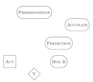
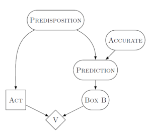
To make this concrete, let’s look at Newcomb’s problem (which has no observations $x$ ). We’ll represent the distribution graphically by drawing boxes for each different thing that Eve knows about.

Predisposition is Eve’s own predisposition for choosing one box or two boxes.
Accurate is how accurate Omega is at predicting Eve. In most forms of Newcomb’s problem, Accurate is very close to 1.
Prediction is the prediction that Omega makes about whether Eve will take one box or two boxes.
Box B is the contents of Box B (either empty or $1 million).
Act is what Eve actually decides to do when presented with the problem.
V is the value that Eve assigns to what she got (in this case, just the monetary value she walked away with).

Some of these boxes are stochastic in Eve’s model, and some are deterministic. Whenever any box changes in value, the probabilities that Eve assigns for all the other boxes are updated to account for this.

So if Eve wants to know $P(one\ box\ \rightharpoonup \ Box\ B\ contains\ \$ 1million;\ x)$ , then Eve will imagine setting Act to “choose one box” and then update her probability distribution for every other node.

The main problem with conditional probabilities as the sole model of the world is that they don’t take into account the way that actions change the world. Since only the statistics of the world matter to Eve, she can’t tell the difference between something being causal and something being correlated. Eve updates probabilities for every box in that picture whenever she imagines doing something different.

That’s actually why she’s willing to pay up to the termite extortionist. Eve can’t tell that whether she pays the extortion has no impact on her house’s termites.

Causal Decision Theory

Causal decision theory is similar to evidential decision theory, but with some added constraints. Carl, who is a causal decider, has a probability distribution to describe the world as well. But he also has an additional set of data that describes causal interactions in the world. In MIRI’s FDT paper, this extra causality data is represented as a graph, and the full model that Carl has about the world looks like $(P(.|x), G)$ .

Here, $P(.|x)$ is again a conditional probability distribution. The causality data, $G$ , is represented by a graph showing causation directions.

Carl’s probability distribution is very similar to Eve’s, but we’ll add the extra causality information to it by adding directed arrows. The arrows show what specific things cause what.

Constructing a hypothetical for this model is a bit easier than it was for Eve. Carl just sets the Act node to whatever he thinks about doing, then he updates only those nodes that are downstream from Act. The computations are performed radiating outwards from the Act node.

We represent this mathematically using the $do()$ operator: $M^{a\rightharpoonup} = P(.|do(a), x)$ .

When Carl imagines changing Act, he does not update anything in his model about Box B. This is because Box B is not in any way caused by Act (it has no arrows going from Act to Box B).

This is why Carl will always two-box (and thus only get the $1000 from Box A). Carl literally cannot imagine that Omega would do something different if Carl makes one decision or another.

Functional Decision Theory

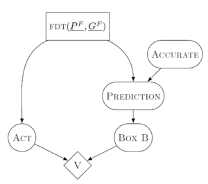
Fiona, a functional decision theorist, has a model that is similar to Carls. Fiona’s model has arrows that define how she calculates outwards from points that she acts on. However, her arrows don’t represent physical causality. Instead, they represent logical dependence.

Fiona intervenes on her model by setting the value of a logical supposition: that the output of her own decision process is to do some action $a$ .

For Fiona to construct a hypothetical, she imagines that the output of her decision process is some value (maybe take two boxes), and she updates the probabilities based on what different nodes depend on decision process that she is using. We call this form of dependence “subjunctive dependence.”

In this case, Fiona is not doing action $a$ . She is doing the action of deciding to do $a$ . We represent this mathematically using the same $do()$ operator that Carl had: $M^{a\rightharpoonup} = P(.|do(FDT(P,G,x))$ .

It’s important to note that Carl conditions on observations and actions. Fiona only conditions on the output of her decision procedure. It just so happens that her decision procedure is based on observations.

So Fiona will only take one box on Newcomb’s problem, because her model of the world includes subjunctive dependence of what Omega chooses to do on her own decision process. This is true even though her decision happens after Omega’s decision. When she intervenes on the output of her decision process, she then updates her probabilities in her hypothetical based on the flow of subjunctive dependence.

Similarities between EDT, CDT, and FDT

These three different decision theories are all very similar. They will agree with each other in any situation in which all correlations between an action and other nodes are causal. In that case:

1. EDT will update all nodes, but only the causally-correlated ones will change.
2. CDT will update only the causal nodes (as always)
3. FDT will update all subjunctive nodes, but the only subjunctive dependence is causal.

Therefore, all three theories will update the same nodes.

If there are any non-causal correlations, then the decision theories will diverge. Those non-causal correlations would occur most often if the decider is playing a game against another intelligent agent.

Intuitively, we might say that Eve and Carl both mis-understand the structure of the world that we observe around us. Some events are caused by others, and that information could help Eve. Some events depend on the same logical truths as other events, and that information could help Carl. It is Fiona who (we think) most accurately models the world we see around us.