Brouwer and the Mountain

A few years ago, one of my friends told me the following riddle:

A mountain climber starts up a mountain at 8am. They get to the top that day, and camp there. In the morning, they start hiking down the mountain at 8am on the same trail.

Is there a time of day at which they’re at the same spot on the trail the second day as they were on the first?

I thought about this a while before finally asking for the answer (which I won’t repeat here). I will say that you don’t have to make any assumptions about hiking speed, rest breaks, or even that the hiker always heads in the same direction.

When I learned about Brouwer’s fixed point theorem, I immediately thought back to this riddle. The answer to the riddle is a straightforward application of Brouwer’s theorem.

It turns out that Brouwer’s theorem is used in all sorts of places. It was one of the foundations that John Nash used to prove the existence of Nash equilibria in normal form games (for which he won the Nobel).

The moral of the story is: the more riddles you solve, the more likely you are to get a Nobel prize.

Why Transform?

I’ve just recently had an epiphany about signal processing. It’s kind of embarassing that it’s taken me so long to realize this, but all the transforms that I’ve been doing in classes are just to make the signal separable from the noise in my data.

That seems pretty simple, so let me back up and explain why it took me so long to realize this. I’ve been taking signal processing classes off and on for about five years now. The classes mostly have focused on a few transforms (fourier and wavelet mostly) and how they can be used to filter an incoming signal. We’ve made low pass filters, high pass filters, and everything in between. It was never quite clear to me why you use the tranform though. You can just do everything in the time domain.

I didn’t put too much thought into that because computations can be easier to do in the frequency domain. What’s convolution in time corresponds to multiplication in frequency. It can be faster to do some calculations in the frequency domain because of that correspondence. I understood that, and thought that I was using some transforms that brilliant people had invented just to speed up their computations. I had no intuition for how they could have devel0ped  the transform. How could they have known the transform would make calculations faster? I put it down to Laplace and Fourier just being more brilliant than me.

What I’ve recently come to realize is that, while Laplace and Fourier were indeed brilliant, their transforms serve a different purpose altogether. The speed up that I got in filter calculations is almost an afterthought to the real purpose of using a transform.

Filters only let through the frequencies that you want. This is obvious when you see plots of filters in the frequency (fourier) domain. I was clear on this from the outset. You use the Fourier transform to select frequencies, gotcha.

For some reason, this knowledge didn’t generalize like it should. I went around saying to myself that filters select different frequencies, and that convolution in time was multiplication in frequency, but I didn’t get that this was the whole point of the transform in the first place. Noise in the time domain is hard to separate from a signal, but in the frequency domain it can be very easy to separate.

And that is the key behind transforms. The real reason you do the transform isn’t so that you can do fast multiplication instead of slow convolution. The real reason to transform a signal to a new domain is because the new domain can make the parts of the signal you’re interested in easier to separate from everything else. That just happens to make the calculations faster too.

This separability comes up in all kinds of signal processing, pattern recognition, and machine learning. A transform may help anywhere where you want to separate one type of thing from another. Making it easier to separate the wheat from the chaff is why you would calculate features before feeding your data into machine learning algorithms.

My understanding of signal processing now revolves around three steps.

  1. Transform the incoming data so that the components you’re interested in are easy to separate from the components you’re not (separate the signal from the noise).
  2. Do whatever calculations you need to in order to get the output that you want.
  3. Transform the output to the domain you need it in; the new domain is usually, but not always, the same as the domain the data had in the first place.

Probability and Logic

When I first started learning math I focused a lot on formal logic and proofs. I had a lot of fun deriving things using induction, proof by contradiction, and simple direct proofs. It’s been a long time since I’ve done much of that, but I find myself thinking a lot about methods of proving things as I learn more about signal processing and statistics.

I spent some time recently studying hypothesis testing and signal detection theory for a classification problem I’m working on at school. What really surprised me about the two things was how similar they were to proof by contradiction. The main ideas in hypothesis testing is

  1. figuring what you want to show (called H1), and
  2. showing that the opposite of that (called H0) is unlikely

This is where the infamous p-value comes from. If you want to show that eating spinach gives people Popeye arms, you start by assuming that it doesn’t. This is called the null hypothesis and is denoted by H0. After you do a lot of measurements on people who have eaten spinach, you figure out how likely are their huge Popeye arms under the assumption that nothing at all has happened. That probability is called your p-value, and if it’s very low then you’ve got your “proof by contradiction”. A low probability that their Popeye arms are due to the null hypothesis indicates that there’s a high probability that something interesting is going on with those cans of spinach.

And because you’re doing statistics, it doesn’t actually prove anything. All it shows is that it’s more likely that spinach has an effect than that it doesn’t. It’s kind of a subtle point, and has led to a lot of mistaken or misleading scientific papers over the past few decades. That’s one of the reasons that a lot of people are calling for different methods of testing hypotheses (such as Bayesian methods [pdf]).

To my mind, Bayesian methods correspond more to a direct proof. That may make it easier to understand and get right, but it doesn’t mean that hypothesis testing’s p-values are useless. There’s room in science for all kinds of methods, just like so many proof methods can be useful. The key is to know your tools and understand their limitations.

And right off the bat we can see one of the main limitations with hypothesis testing using p-values. Since you’re doing something akin to “proof by contradiction”, you can’t compare different options very easily. You can say things like “Popeye arms are likely to be cause by eating spinach with p-value .02” or “Popeye arms are likely to be caused by excessive mastubation with p-value .03”, but you can’t compare those two hypotheses. One may be more likely to be true than the other, but you can’t easily tell just using p-values. Since you’re only comparing individual hypotheses to the null hypothesis, you don’t know how the hypotheses relate to each other.

That said, hypothesis testing and p-values can be a strong technique when used on the right problem; just like proof by contradiction.

Surfing the shockwave

I’m went on a road trip to San Diego a few weeks ago. When I got there I went straight to the beach for some hard core surfing. It was cloudy, but I ended up having fun anyway.

The thing about surfing is that it really makes you think about waves. Is this next wave worth catching? What about that one? But when I’m just sitting out in the water waiting for a wave, I start thinking about waves themselves.

The question that came to my mind was: why do waves crest as the get closer to the beach? When waves are far from shore, they approximate a sine wave. The amplitude of the wave is the distance away from sea level.

A wave in deep water.
The equation for this wave is D = D_0 + A\sin(\omega t-kx) . D here is depth, and D_0 is sea level. A is the maximum height of the wave, \omega is the angular frequency 2\pi f , t is the time, k is the wave number 2\pi /\lambda , and x is the distance away from shore.

As you can see in that equation, the depth varies with time and distance. The distance here doesn’t really have anything to do with the beach though. What could be causing the waves to break? So I did some research.

According to wikipedia, waves on a beach are shock waves. That’s right, just like the shock wave from a plane. These shock waves work slightly differently.

Here’s what happens:

The speed of a wave in water depends on the depth of the water. When a wave is in deep water far from the beach, slight changes in depth due to the wave itself have a tiny effect. When the wave nears the beach, the water is shallower and the wave itself has a larger effect.

Near the beach, the peaks of a wave travel faster than the troughs. That means that high points catch up to low points. The wave loses its sinusoidal shape and starts turning into a sawtooth wave, and sawtooth waves have discontinuities. Discontinuities manifest themselves strangely in nature. In this case, they’re manifested as the crests of the wave.

Shockwave
The shock appears as the wave travels to the right.

I modeled this by changing the wave number, k as a function of the previous amplitude. Basically, I assumed that the water got shallower as the wave moved to the right. Since I only changed the wave number and left the frequency the same, the speed of the wave changed with amplitude.

The problem with my approach is that I changed wave speed linearly, and shock waves are by nature a non-linear problem. My model worked well for small changes in the wavespeed, but large changes caused a breakdown that manifested itself as spurious peaks. I could make a better model, but right now I don’t really feel like going through all of the calculus that would require. The KZK equation is for physicists.

Model Breakdown
You can’t model a non-linear process very well with linear tools.

Find the code here.

Opening Doors

I ran into an interesting math puzzle while trawling the blag-o-sphere today.

One hundred students line up to walk by one hundred closed lockers. The first student walks by opening every locker that is closed. The second student then walks by and opens every second locker that is closed and closes every second locker that is open. The third student does the same for every third locker and the nth student does the same for every nth locker.

After all the students have walked by the lockers, how many lockers are open?

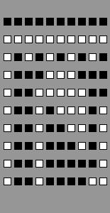
I thought about this for a while, but I was having some trouble visualizing what was happening. In the end, I decided to graph it to see what was happening. I wrote up a quick Processing sketch and looked at a smaller version of the problem. My smaller version had only ten lockers and ten people who run through them.

Timeline of ten lockers being toggled

Once you’re looking at the picture, the answer the question is obvious. I’m not very satisfied with this method of solving the problem. It seems inelegant, and is purely a brute-force approach.

Another way to approach the problem is see if there is a closed form solution for any given door. If we had that, we could solve for the state of each locker and sum them up. Unfortunately, I think this comes down to a factoring problem. If the locker number has an even number of factors, then it is closed. If it has an odd number of factors, it is open. Interestingly, since most of the lockers remain closed it seems that most numbers have an even number of unique factors. That doesn’t really help explain the problem though.

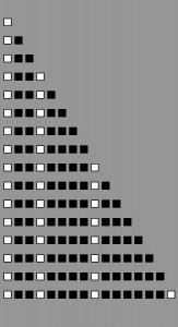
Solutions upto 16 Lockers

So if I can’t find a closed form solution to the state of each locker, what other patterns can I see? By looking at the solutions for different numbers of lockers, I see that total number of lockers needed to give a certain number of opens follows some kind of power function. Looking at the first sixteen solutions shows that if I want n open lockers, then I need 2^n total lockers.

This is more like it. Now when someones asks about 100 lockers, I can find a solution quickly. What squared is 100? It’s 10 of course, so there are 10 open lockers after this sequence of events has been applied to 100 lockers. For any number, n, of lockers, the number of open lockers after n people have run though them is ?n rounded down.

So now I have my answer. I just need a reason. Why is it the case that the open doors follow this pattern? What that really boils down to after looking at it for a bit is the question: why are the only doors left open doors that are the square of a number? Does this mean that only square numbers have an odd number of unique factors?

Square numbers are the only numbers that have an odd number of unique factors because factors can come in pairs. With a square number, one of those pairs is made up of two of the same number, and in this situation that can only count as one toggle, not two.

So take locker number 10 for example. It has factors 1, 2, 5, 10. In this case 1 goes with 10 and 5 goes with 2. They cancel each other out and the locker stays closed.

The number 9, on the other hand, has factors 1, 3, 9. Here the 1 and the 9 cancel each other out, but the 3 doesn’t have anything to cancel it out. The locker remains open.

It turns out that getting sidetracked about closed form solutions for each individual door actually did provide the hint to understanding the problem.

You can get the code I used for my images here.

Counting eggs before they’re cooked

I eat a lot of eggs. Maybe three times a week, I’ll make myself an egg burrito for breakfast. I also tend to eat a lot of omelets for dinner. That’s six eggs a week for breakfasts, plus maybe four more for dinners. I eat a lot of eggs, which means I got through a lot of egg cartons.

In the mornings, when I’m standing bleary eyed in front of the stove waiting for my eggs to cook, I often amuse myself by placing the remaining eggs into the carton in some symmetric fashion. I do this so often that I’ve started eating even numbers of eggs at a time, just to make sure I can put away the rest of the eggs symmetrically.

When I started doing this, I generally just tried to arrange them with symmetry about the x-axis. In this case, the x-axis divides a dozen egg carton in half hot-dog style (even though I eat lots of eggs, I don’t really buy the larger cartons). Arranging eggs in this manner is easy, because all you do is organize the bottom row in the same way as the top row.
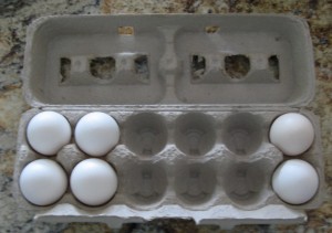
Symmetry about the x-axis

Organizing eggs symmetrically got me thinking about how many ways I could actually pack them. For x-axis symmetry, I really only care about the top row. After I set the top row, the bottom row is uniquely defined. So if I have some even number of eggs, the number of ways I can put half of them into the top row is the same as the number of ways I can organize the eggs symmetrically.

It turns out that counting the number of ways I can put (for example) 2 eggs into 6 spots is given by the choose function. The choose function, (n choose k), is defined as the number of ways that you can pick k things from n possibilities. That’s exactly what I’m doing when I put eggs into a carton: I’m choosing 2 out of 6 possible places to put eggs.

This means that if I have 2n eggs left, for 0<=n<=6, there are (6 choose n) ways of organizing the eggs symmetrically. If I try every possibility each morning starting on the day that I got them (not on the day I first ate them) then I’ll have tried (6 choose 6) + (6 choose 5) + … = sum from i = 0 to 6 of (6 choose i).

Plugging this into Python, I get:

>>> from math import *
>>> sum = 0
>>> for i in range(7):
... sum += factorial(6)/(factorial(i)*factorial(6-i))
...
>>> sum
64

This is 64 possible combinations, just for vertical symmetry.

After a few months of eating eggs, I’d pretty much covered all of those. To make it a bit more interesting, I decided to go for horizontal symmetry instead. You still end up dividing the eggs and placing half of them in the left side of the carton. The right side is just a mirror of the first. At first, this seemed like it would be more interesting because instead of one row of eggs, I actually have three rows of two.

Symmetry about the y-axis

Unfortunately, the math works out exactly the same. There are still only six positions to place the eggs. This time the six are on one side, rather than on the top. While the positions might look slightly more interesting, there are the same number of them.

The last place to look for interesting symmetries in my dozen-egg carton is rotational. In this case, the carton would look the same if I rotated it 180 degrees. This only happens if the top right quadrant is the mirror of the bottom left. Same goes for top left and bottom right. So I’ve got my even number of eggs, and I can then divide them and put them however I want in the left quadrants, which defines the positions in the two right quadrants.
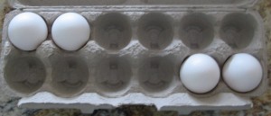
Symmetry about the origin

This is exactly the same as with both other forms of symmetry; the only change is how the new egg positions are defined.

The last thing that I’m interested in here is the combination of all three forms of symmetry. A carton packing that is symmetric about the x-axis and y-axis is also symmetric about the origin, but not all packings that are symmetric about the origin are also symmetric about both axes.
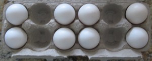
Symmetry about the x- and y-axes

To create symmetry about both axes, we only have choices in a single quadrant. Once one quadrant is packed, all three other quadrants are explicitly defined. This means that the total number of eggs has to be divisible by 4, not just 2. We can only do this with 12, 8, 4, and 0 eggs.

With 12 eggs and 0 eggs, there isn’t even a choice. Both those options give us a single method of creating symmetries. The 8 egg option means that there will be two eggs in each quadrant, for a total of (3 choose 2) symmetry options. The 4 egg option means that there’s one egg in each quadrant, giving us (3 choose 1) symmetry options.

(3 choose 2) = 3
and
(3 choose 1) = 3

This is because if you’re putting one object into three places, there are three possible ways to do it. If you’re putting two objects into three places, that’s the same as leaving one object out of three places. Thus the two are the same.

The total number of carton packings that are symmetric about both axes and the origin is then 1 + 1 + 3 + 3, or 8.

Now that I’ve actually worked out how many symmetries there are, I may get around to writing a program to generate them all. Sounds like I’m going to get more practice with Processing.