LiDAR sensors are very popular in robotics, and work a lot better than cameras for localization and mapping. This is largely because you get the distance to everything the LiDAR sees automatically. With cameras (monocular or stereo), you have to do a lot of math to figure out far away things are and whether two things are spatially separated.

How are LiDAR actually used though? Once you have a LiDAR, how do you convert the data it spits out into a map that your robot can use to get around? One of the more popular algorithms for this is LOAM (LiDAR Odometry and Mapping). There are a few different open source implementations, but the most popular seem to be A-LOAM and Oh My Loam. I’m thankful to both of them for helping me to understand the paper.

Let’s dive into how LOAM works.

Note that some of the details of the algorithm are slightly different depending on what implementation you’re looking at, and the below is just my understanding of the high level algorithm.

Point Clouds

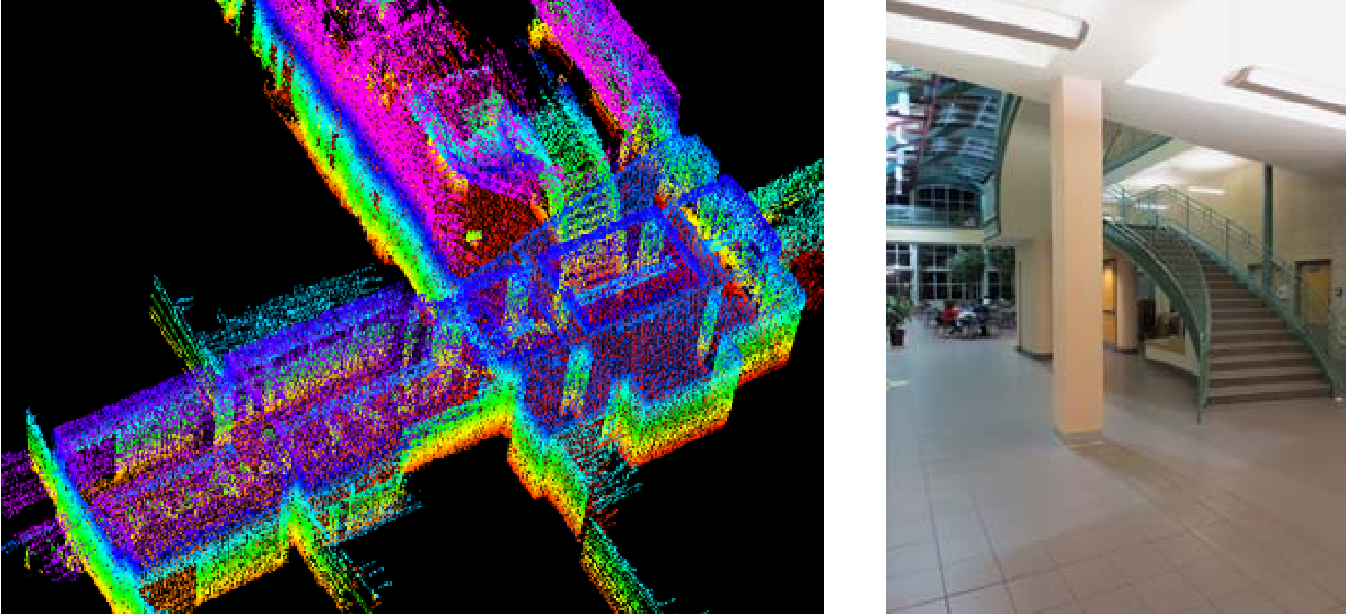
Before understanding how LOAM works, let’s learn a bit more about LiDAR data in general. The most popular way of storing LiDAR data is as a Point Cloud. This is simply a vector of the 3D points the sensor returns. In general, a LiDAR will return some measurements of azimuth, elevation, and distance for each object relative to the LiDAR itself. From these, you can calculate the X, Y, and Z positions of stuff in the real world. A point cloud is just a collection of these points, and if you’re using something like the Point Cloud Library then it will come along with a lot of utilities for things like moving the points around in space, registering points to new reference frames, and controlling the density of points in space.

These functions to shift points around are critical, because your LiDAR is going to be moving as you map. Every point that comes out of your sensor is defined in the reference frame of the sensor itself, which is moving around in the world. To get our map, we’ll want to to be able to take a point that’s defined relative to a sensor and shift it to where it should be in some fixed world plane.

We can use some functions from PCL to shift those clouds, but before that we need to figure out how they should shift. We do this by using LOAM to calculate how the sensor has moved between different LiDAR frames.

Usually point clouds are assumed to be unordered. We’re going to stick some additional information into our cloud before using it. Specifically, we’re going to keep track of which laser the data came from. We do this because most LiDARs have different azimuth resolution than elevation resolution. Velodyne’s VLP-16, for example, has 0.2 degrees of resolution in azimuth and 2 degrees of resolution in elevation. LOAM uses points differently if they’re aligned in the high resolution direction, and by tracking which laser the points came from we can inform LOAM about which direction is the high resolution direction.

Maps

I’m apparently old now, because when I hear the word map I think of one of those fold-out things we used on road trips when I was a kid in the pre-smartphone era. The kind of map that takes up 10 square feet and covers the entire continental US. These road maps are abstract pictures of the world with included semantic meaning. They have labels. You can see what places are cities, where national parks are, and figure out if you can make it to the next rest stop.

When people talk about SLAM maps, they’re not talking about this kind of thing. The kind of map produced by LOAM and other SLAM techniques doesn’t have any semantic meaning. You could have a robot map your whole house, and LOAM wouldn’t be able to tell you where your kitchen was or the distance from your bedroom to the bathroom. What the produced map can tell you is what the 3D geometry of your house looks like. What places can the robot navigate to, as opposed to places that are occupied by your favorite chair.

The lack of semantic meaning for SLAM maps tripped me up when I was first learning about them. I kept seeing pictures of LiDAR points projected in space, then asking where the map was. The projected LiDAR points were the map! If you want to know what room has the oven, if you want semantic meaning, you’ll have to run your map through a higher level process that recognizes things like ovens (people are working on it).

The LOAM algorithm is going to take in point clouds generated by LiDAR as the sensor moves through space. Then LOAM is going to spit out one big point cloud that represents the geometry of the whole space. This is enough for a robot to avoid hitting things, plan routes between two points, and measure the distance between things (but it won’t know what those things are). In order to collate the series of point clouds the sensor spits out into one big map, LOAM needs to do two things:

1. Figure out how the LiDAR has moved in between one scan and the next
2. Figure out what points to keep in the map, and move them all to the right position relative to each other 

These two steps are the L and the M in SLAM. By using sensor data to figure out where the robot is (localization), subsequent sensor readings can be aligned with each other to create a full map. LOAM does the localization part via LiDAR odometry. In other words it figures out from comparisons of one cloud to the next how the sensor has moved between when those clouds were captured.

Odometry

Doing odometry just means that you calculate the relative locations of the sensor given two point clouds. This gives you the motion of the robot between when the point clouds were made (also called ego-motion).

People are pretty good at looking at two pictures and estimating where they were taken from, but making a computer do this is pretty complicated. The (non-ML) state of the art is to find distinguishing points in the image (or point cloud). If you find the same distinguishing points in your second frame, you can use the difference in position of the point in the two scans to figure out the location difference of the sensor. This depends on a few different assumptions:

1. interest points won’t get confused for each other (at least not very often)
2. interest points don’t move around (so don’t use a dog in the frame as an interest point)

With LOAM, we’ll just assume that there aren’t any people, pets, or other robots in the scene. That satisfies assumption 2. How do we make sure that the distinguishing points won’t get confused with each other? And what is a distinguishing point anyway?

Feature Points

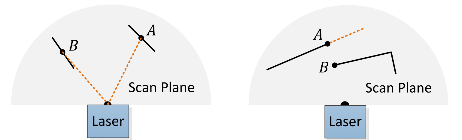
Distinguished points in an image or point cloud, generally referred to as feature points, are individual points in an image or point cloud that you can identify using local characteristics. For an image, they’re individual pixels. For a point cloud, individual laser returns. What makes them good features is that the other points around them have distinct spatial or color characteristics. Different algorithms (such as SIFT or SURF in camera-vision) use different characteristics. LOAM’s characteristic of choice is something they call curvature. By looking at how much the points curve through space, LOAM can identify flat planes (like building walls or floors) and edges (like table edges or places where one object is in front of another).

LOAM’s curvature measurement is calculated by looking only at points that are from the same “scan”. In this case, a scan means from the same laser and the same revolution. For a Velodyne, one revolution of the device produces a single set of 16 scans (or up to 128 if you have the expensive one). By only examining points in the same scan, LOAM’s curvature knows that the points should have the same angular distribution and lie in a plane (though that plane may be skew to X/Y/Z dimensions that define your world).

To calculate curvature, you pull all the points out of your incoming point cloud that came from the same scan. Next, you sort these spatially. You can get this spatial sorting by just looking at when the points were reported by the sensor, you don’t actually have to do any geometry for this step. For example, if you’re looking at circles reported by a single laser in a VeloDyne as your scan, then you can just order the points by the time they come in and have a spatial ordering as well.

After the points are ordered spatially, you calculate the curvature of every point. This curvature is calculated using only the 5 points on either side of the point you’re looking at (so 10 points plus the center point). You look at how far each nearby point is from the one you’re looking at, and sum those distances. High curvature points will have a high sum, low curvature points will have a low sum. There’s a pretty good code sample for this in the Oh My LOAM repo.

Not every curvature point will be considered to see if it’s a good feature. In particular, the following points are filtered out:

1. points that are on a surface that’s almost parallel to the laser beam
2. points that are on an edge that could be occluding something else

After being calculated, curvature values are sorted. Maximal curvature points are then selected as edge features and minimal curvature points are selected as plane features. Since it’s possible that all the maxima (or minima) are in one place, the scan is split into four identically sized regions. Then each region can provide up to 2 edge points and 4 plane points. Curvature points are selected as features only if they are above (below for planar points) a set threshold.

At the end of this procedure, you should have two distinct point clouds: the edge cloud and the flat cloud. (In LOAM software, there’s some terminology overlap. The words “surface”, “flat”, and “plane” all generally refer to the same set of points. Similarly, “edge” and “corner” both refer to the same set of points. I’ll use these terms interchangeably)

Correspondences

The first time you get a point cloud out of your sensor, you’ll just calculate a bunch of features and fill up an edge cloud and a flat cloud. The second time, you’ll have an old frame to actually compare the new features to. Now you can do odometry by comparing the new features to the old features. If you compare two lidar clouds to each other, you can calculate how the sensor moved between those frames, which is called the transformation.

For each feature point in your current edge and flat clouds, you find the nearest point in the the prior edge and flat clouds.

Finding correspondences is kind of tricky, and it involves repeatedly trying to find the best correspondence. This is done using an algorithm called Iterative Closest Point (or ICP).

In LOAM’s ICP, you do the following:

1. match corners between this frame and the last one using a guess-transform
2. match surfaces
3. using those matches, revise your transformation from the current frame to the last one
4. figure out how good the guess-transformation is, and improve it
5. repeat 3&4 until you have a good enough transformation

Matching points

Matching points is done by looking at each point in the edge cloud (or flat cloud and, for each point:

1. guessing at how to transform it to the pose of the prior frame
2. then finding the closest point to where your corner would be in the prior frame’s corners.

Guessing how to transform the point you’re looking at is tricky. This is basically the transformation you want to find anyway, that’s why you’re finding the correspondences in the first place. Finding correspondences is therefore a game of guess and check. To speed things up, we’ll make the best guess we can: the transformation between this frame and the last one is the same as between the last and the one before that. In other words, we think the robot is moving in a fairly consistent way. That’s not true, but it’s a good start assuming we’re sampling lidar frames fairly quickly.

If we don’t have a prior transformation to use as our guess, we can just assume that there’s been no motion (so we’d use an identity transformation).

After we’ve done our transformation of our candidate point to where it would have been before we moved, our next step is to find it’s corresponding point from the last cloud. This can be done using any nearest neighbor algorithm (kNN is a good choice).

For the corner points, we actually find the two nearest points to our candidate. You can draw a line through any two points, so by finding the nearest two from the prior frame we can evaluate whether our new point is on that same edge line. We don’t care if our new point is exactly the same as the prior points (it probably won’t be the same spot in space). We just care that it’s looking at pretty much the same edge that the prior ones were looking at.

We end up doing the above process for every edge point we found, comparing them to the prior frame’s edge points.

Then we do the process for every flat point we found, comparing them to the prior frame’s flat points. For the flat points, we actually find the nearest three points in the prior frame’s set of flat points. This is because you can draw a plane through any three points, and we want to see if our new candidate flat point is on the same surface (not necessarily if it’s the exact same spot in space as a prior point).

We’ll need the following information for each point going forward:

1. the point position in the current lidar frame (not adjusted using our guess-transformation)
2. the corresponding points (for the line or plane) in the last lidar frame
3. the transform we used to find the correspondence

Now we just need to know how good our candidate transformation was.

Evaluating the Match

We now have a list of points and the things we think they match to (lines or planes). We also have a single transformation that we think we can apply to each point to make them match. Our next step is to update that transformation so that the matches we think we have are as good as possible.

The update step for most open source implementations that I’ve seen is done using the Ceres Solver. Improving the transformation is formulated as a non-linear least squares optimization problem. The Ceres library is used to solve a least-squares optimization using the Levenberg-Marquardt algorithm.

The optimization being solved by Ceres is the distance between the correspondence points and the new lidar points that are corresponded to, after transforming the latter. The solution to this optimization problem is a transformation, and if our original guess was good then the solution will be pretty close to our guess. Either way, we’ll use the solution given by the Ceres Solver as our new guess for the transformation.

Refining the candidate transform

The sections we just saw for correspondences (finding the correspondences, optimizing the guess-transform) were just a single iteration of the Iterative Closest Point algorithm. Once you’ve done this once, your guess transform should be better than it was.

With a better guess transform, you could probably get better initial correspondences, which would lead to a better optimized transform. So we just repeat the whole process a few times.

Ideally, after you iterate this process enough the guess-transformation stops changing. At that point, you can be pretty sure you know how the sensor moved between the last frame and this frame. Congratulations, you’ve just performed odometry.

Now throw away the old point cloud and use your new point cloud as the comparison point once the next frame comes in. Repeat this process ad-nauseum to track how the robot moves over time. The odometry pipeline can happen in its own thread, completely independently of any mapping.

Mapping

Figuring out how the robot moves is useful, but it would be even more useful to have a complete voxel style map of the environment the robot moves through. The output of the odometry step is the single-step transform between one LiDAR frame and the next, and a cloud of feature points used to calculate that transform.

You can use that single-step transformation to update a “global transformation” that would place the point cloud relative to the robot’s starting position. The naive thing to do is to transform the feature points from the odometry step using that global transform, and then just save them all into the same point cloud. You’d think that doing this would result in the voxel grid you want, but there are some hiccups.

Odometry is optimized to be fast, so it only compares incoming LiDAR frames to the data in the immediately prior frame. That’s useful for getting a pretty good estimate of how the robot moves from frame to frame, but it’s going to be inaccurate. You only have one frame’s worth of points to compare with when you’re generating your odometry transform, so the closest points you use during ICP may not be all that close. Instead of using odometry output clouds directly for a map, we can run ICP a second time on a larger set of points. That let’s us refine the position of the new points before inserting them, resulting in a much more accurate map.

The reason we don’t do this step with odometry is, again, because odometry needs to be fast. The original LOAM paper runs odometry at 10x the speed of mapping. The Oh My Loam implementation just runs mapping as fast as it can, but then ignores any LiDAR points coming from the odometry stage while it’s processing. This means that it silently drops some unknown number of LiDAR points and just accepts incoming data when it’s able to handle it.

The mapping stage is almost the same as the odometry algorithm that we went over above. Here are the differences:

1. the candidate transform used in the first stage of ICP is the output of odometry (so we have a pretty good starting transform)
2. instead of comparing each incoming point to a single line or surface in the map (as odometry does), the map grabs a bunch of nearest neighbor points to compare to. The exact number is a configurable parameter, but by comparing to a bunch of points you can get a better idea of the exact geometric feature your incoming point belongs to
3. the optimization criterion for Levenberg-Marquardt is tweaked a bit to account for the additional points (item 2)
4. instead of only having a single LiDAR frame to look for neighbor points in, you can look for neighbors in the entire map

In practice, you actually take a sub-section of the map to look for your neighbors in to speed things up. No need to look for neighbor points a quarter mile away if your LiDAR range is only a few hundred feet.

Other than the above differences, the ICP algorithm proceeds almost identically to the odometry case. Once you have a fully refined transformation for the incoming points, you can use PCL to move the point to where it should be in space. This amounts to making its location be relative to the starting point of the robot’s motion, rather than relative to the LiDAR position when the point was detected. Then the point is inserted into the map.

The map itself is a collection of the surface and edge points from prior LiDAR frames. A lot of those points are likely to be close to each other, so the map is down-sampled. This means only points far enough away from other points are stored. In the paper, they set this distance as 5cm. The points themselves are stored in a KD-tree, which is a fast way of storing point clouds.

Two great tastes that taste great together

By doing odometry as close to real time as you can, you can track how your robot is moving through space. By doing a separate mapping stage that takes that odometry information into account, you can spend a lot of time making an accurate map without sacrificing your position estimate. Separating these tasks makes them both perform better.

In particular, odometry is important for things like motion planning that may not need access to the map. You can’t stop odometry while you wait for your map to compute. But odometry by itself can be very noisy, and you wouldn’t want something that needs a map depend only on lidar-odometry information for environment estimates.

There are a lot of ways to improve on this type of algorithm. One of the more obvious ones is to supplement your odometry stage with another sensor. If you have an IMU measuring accelerations, you can use those seed your initial transform estimate in your lidar-odometry step.