Reading SD cards with the Arduino

About a year ago, I got my friend Ryan an Arduino for his birthday. We futzed around with it for a while trying to come up with a good project, and in the end we decided to try to read an SD card.

We didn’t really have a reason for it, it just seemed like an achievable goal for a first Arduino project. I seem to recall that we wanted to understand SPI, and Ryan wanted to implement SPI in software. After about a month of weekly meetings, we were still trying to figure out the SD card SPI standard. We’d made some progress with the initialization routine for the card, but the CRC functions had us completely stumped.

In the end, my friend moved to NYC and I completely forgot about the project.

Fast forward to a month ago and I’m looking into ways to get my Arduino to play some sound files for a robotics project. When I stumbled on the Adafruit Waveshield, I also found an answer to my SD card questions. The Waveshield comes with a library to read SD cards. It didn’t take me long to get it working with the hardware I had on hand.

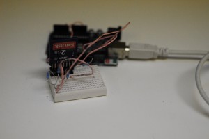
I wrote up a quick script to read and display the contents of a file, then hooked up my SD card. I didn’t have an SD slot handy, so I soldered some headers together into a nice holder. It may be hard to tell from the picture, but I used three sets of headers. One on the bottom sandwiched by two on the top. The top two also clamp onto the SD card.

Three headers can sandwhich an SD card

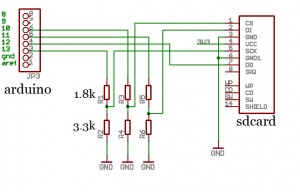
This allowed me to connect the SD card as shown in this schematic. The resistors are there to act as voltage dividers. The SD card needs 3.3 V signaling, but the Arduino provides 5 V signaling. In the Adafruit Waveshield, they use buffers to do the level conversion. Voltage dividers are quick and dirty, but probably not the best solution.

The sketch I wrote required me to add the Adafruit library to my library folder, as shown here.

Once I had everything hooked up, it worked great. The only problem I ran into while putting this together was the formatting of the SD card. The SD library expects FAT16 formatting, which means that the naming conventions for files are pretty strict. Filenames have to be at most eight characters before the “.”, and file extensions can only be three characters.

Connected SD card

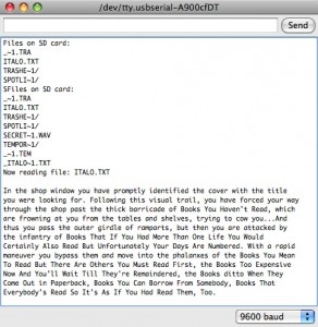
Output text from Arduino SD reader

I think I might put together a little R-2R DAC and make myself a quick and dirty music player.

Code for this is as follows:

#include <FatReader.h>

SdReader card;
FatVolume vol;
FatReader root;
FatReader file;

void setup() {
  Serial.begin(9600);
  if (!card.init()) {
   Serial.println("can't initialize card"); 
  }
  if (!vol.init(card)) {
    Serial.println("can't initialize volume"); 
  }
  if (!root.openRoot(vol)) {
    Serial.println("can't open directory"); 
  }
  
  Serial.println("Files on SD card:");
  root.ls();
}

char filename[] = "ITALO.TXT";

void loop() {
  if (!file.open(root, filename))
  {
     Serial.print("failed to open file");
     Serial.println(filename); 
  }
  char letter;
  
  Serial.print("Now reading file: ");
  Serial.println(filename);
  while (file.read(&letter, 1) == 1) {
   Serial.print(letter);
  }
  
  while (1) {}
}

Surfing the shockwave

I’m went on a road trip to San Diego a few weeks ago. When I got there I went straight to the beach for some hard core surfing. It was cloudy, but I ended up having fun anyway.

The thing about surfing is that it really makes you think about waves. Is this next wave worth catching? What about that one? But when I’m just sitting out in the water waiting for a wave, I start thinking about waves themselves.

The question that came to my mind was: why do waves crest as the get closer to the beach? When waves are far from shore, they approximate a sine wave. The amplitude of the wave is the distance away from sea level.

A wave in deep water.
The equation for this wave is D = D_0 + A\sin(\omega t-kx) . D here is depth, and D_0 is sea level. A is the maximum height of the wave, \omega is the angular frequency 2\pi f , t is the time, k is the wave number 2\pi /\lambda , and x is the distance away from shore.

As you can see in that equation, the depth varies with time and distance. The distance here doesn’t really have anything to do with the beach though. What could be causing the waves to break? So I did some research.

According to wikipedia, waves on a beach are shock waves. That’s right, just like the shock wave from a plane. These shock waves work slightly differently.

Here’s what happens:

The speed of a wave in water depends on the depth of the water. When a wave is in deep water far from the beach, slight changes in depth due to the wave itself have a tiny effect. When the wave nears the beach, the water is shallower and the wave itself has a larger effect.

Near the beach, the peaks of a wave travel faster than the troughs. That means that high points catch up to low points. The wave loses its sinusoidal shape and starts turning into a sawtooth wave, and sawtooth waves have discontinuities. Discontinuities manifest themselves strangely in nature. In this case, they’re manifested as the crests of the wave.

Shockwave
The shock appears as the wave travels to the right.

I modeled this by changing the wave number, k as a function of the previous amplitude. Basically, I assumed that the water got shallower as the wave moved to the right. Since I only changed the wave number and left the frequency the same, the speed of the wave changed with amplitude.

The problem with my approach is that I changed wave speed linearly, and shock waves are by nature a non-linear problem. My model worked well for small changes in the wavespeed, but large changes caused a breakdown that manifested itself as spurious peaks. I could make a better model, but right now I don’t really feel like going through all of the calculus that would require. The KZK equation is for physicists.

Model Breakdown
You can’t model a non-linear process very well with linear tools.

Find the code here.

Opening Doors

I ran into an interesting math puzzle while trawling the blag-o-sphere today.

One hundred students line up to walk by one hundred closed lockers. The first student walks by opening every locker that is closed. The second student then walks by and opens every second locker that is closed and closes every second locker that is open. The third student does the same for every third locker and the nth student does the same for every nth locker.

After all the students have walked by the lockers, how many lockers are open?

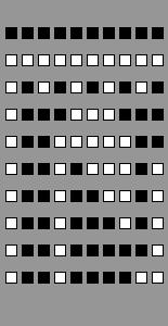
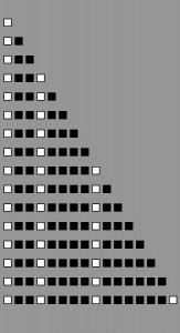
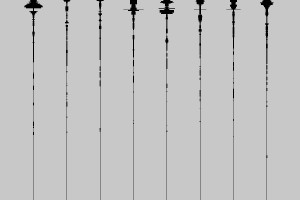
I thought about this for a while, but I was having some trouble visualizing what was happening. In the end, I decided to graph it to see what was happening. I wrote up a quick Processing sketch and looked at a smaller version of the problem. My smaller version had only ten lockers and ten people who run through them.

Timeline of ten lockers being toggled

Once you’re looking at the picture, the answer the question is obvious. I’m not very satisfied with this method of solving the problem. It seems inelegant, and is purely a brute-force approach.

Another way to approach the problem is see if there is a closed form solution for any given door. If we had that, we could solve for the state of each locker and sum them up. Unfortunately, I think this comes down to a factoring problem. If the locker number has an even number of factors, then it is closed. If it has an odd number of factors, it is open. Interestingly, since most of the lockers remain closed it seems that most numbers have an even number of unique factors. That doesn’t really help explain the problem though.

Solutions upto 16 Lockers

So if I can’t find a closed form solution to the state of each locker, what other patterns can I see? By looking at the solutions for different numbers of lockers, I see that total number of lockers needed to give a certain number of opens follows some kind of power function. Looking at the first sixteen solutions shows that if I want n open lockers, then I need 2^n total lockers.

This is more like it. Now when someones asks about 100 lockers, I can find a solution quickly. What squared is 100? It’s 10 of course, so there are 10 open lockers after this sequence of events has been applied to 100 lockers. For any number, n, of lockers, the number of open lockers after n people have run though them is ?n rounded down.

So now I have my answer. I just need a reason. Why is it the case that the open doors follow this pattern? What that really boils down to after looking at it for a bit is the question: why are the only doors left open doors that are the square of a number? Does this mean that only square numbers have an odd number of unique factors?

Square numbers are the only numbers that have an odd number of unique factors because factors can come in pairs. With a square number, one of those pairs is made up of two of the same number, and in this situation that can only count as one toggle, not two.

So take locker number 10 for example. It has factors 1, 2, 5, 10. In this case 1 goes with 10 and 5 goes with 2. They cancel each other out and the locker stays closed.

The number 9, on the other hand, has factors 1, 3, 9. Here the 1 and the 9 cancel each other out, but the 3 doesn’t have anything to cancel it out. The locker remains open.

It turns out that getting sidetracked about closed form solutions for each individual door actually did provide the hint to understanding the problem.

You can get the code I used for my images here.

How dense are your palindromes?

A man, a plan, a canal, Panama.
Bombard a drab mob.
Drab as a fool, aloof as a bard.

Palindromes are strings that can be read the same backwards as forwards. The most common palindromes are words or sentences, but palindromes can be made from any set of characters. Lately I’ve been interested in palindromic numbers, which are numbers (like 1221 and 5567655) where the the nth digit from the beginning is the same as the nth digit from the end.

Palindromic numbers are pretty easy to generate. Just choose a length for the number, then choose some digits for the first half of the number. Mirror those, and you’ve got a number. They’re easier to make than palindromic sentences, because numbers don’t have to make any kind of logical sense. They’re kind of like my symmetric egg basket problem, where choosing one half of a solution defines the other half.

In text, palindromes are kind of rare. Palindromes that actually make sense are rarer still. I wanted to see how rare palindromes are in the natural numbers. It turns out that the density of palindromic numbers decreases exponentially as the magnitude of the number increases.

Every single one digit number is a palindrome. There are nine two digit palindromes (the multiples of 11). Three digit palindromes start to get a little more interesting. Any combination of two digits leads to a palindrome of three digits by copying the first digit as the third. This puts the number of three digit palindromes at 9*10 = 90. There are nine choices for the first digit (we exclude zero) and ten choices for the second digit. Four digit palindromes can be counted in the same way, since instead of copying the first digit you copy both first two.

Continuing on in this way, we can find the percentage of numbers of each order of magnitude that are palindromes:

1 digit: 100%
2 digits: 10% (9 palindromes in 90 numbers)
3 digits: 10% (90 palindromes in 900 numbers)
4 digits: 1% (90 palindromes in 9000 numbers)
5 digits: 1% (9*10*10=900 palindromes in 90000 numbers)
6 digits: .1% (900 palindromes in 900000 numbers)
7 digits: .1% (9*10*10*10=9000 palindromes in 9 million numbers)

Every two orders of magnitude that we go up decreases the percentage of palindromes by an order of magnitude. The number of palindromes only increases with two jumps in the size of the number, but the total number of numbers increases with each jump in the size of the number. This is why the percentage of palindromes will slowly decrease.

Just for fun, I also decided to compare palindromes in one base to palindromes in another. I wrote a python script that would compare decimal palindromes to their hex equivalent and report any hex values it found that were also palindromes.

#check decimal palindromes for hex palindromes

def convHex(decimal_string):
    hex_string = str(hex(int(decimal_string)))[2:]
    is_palindrome = True
    for i in range(len(hex_string)):
        if hex_string[i] != hex_string[-(1+i)]:
            is_palindrome = False
        #end if
    #end for
    if is_palindrome:
        return [int(decimal_string)]
    else:
        return []
    #end if
#end def convHex(decimal_string)


double_palindromes = []
for i in range(1,10000):
    #even number of digits
    palindrome = str(i) + str(i)[::-1]
    double_palindromes.extend(convHex(palindrome))
    #odd number of digits
    palindrome = str(i) + str(i)[-2::-1]
    double_palindromes.extend(convHex(palindrome))
#end for

double_palindromes.sort()

for i in double_palindromes:
    print i, hex(i)

Again, all one digit numbers are palindromes for every base. Since hex has all the single digits that decimal does, all single digit decimal palindromes are palindromes in hex as well. After that, the numbers that are palindromes in both bases get far rarer.
Here’s the list of all numbers up under 9 digits long that are palindromes in both decimal and hex bases:

1 0x1
2 0x2
3 0x3
4 0x4
5 0x5
6 0x6
7 0x7
8 0x8
9 0x9
11 0xb
353 0x161
626 0x272
787 0x313
979 0x3d3
1991 0x7c7
3003 0xbbb
39593 0x9aa9
41514 0xa22a
90209 0x16061
94049 0x16f61
96369 0x17871
98689 0x18181
333333 0x51615
512215 0x7d0d7
666666 0xa2c2a
749947 0xb717b
845548 0xce6ec
1612161 0x189981
2485842 0x25ee52
5614165 0x55aa55
6487846 0x62ff26
9616169 0x92bb29
67433476 0x404f404
90999909 0x56c8c65
94355349 0x59fbf95
94544549 0x5a2a2a5

Wikipedia has a lot more information on palindromic numbers. Apparently they’re pretty common in mathematical riddles and puzzle challenges.

Toy Economies

I went to Ada’s Books last week. They had a lot of textbooks, which I wasn’t too interested in. They also had a lot of science books, which I wasted half my day (alright, just 20 minutes) perusing. I ended up buying Group Theory in the Bedroom. It’s a collection of essays some guy wrote for a variety of science magazines.

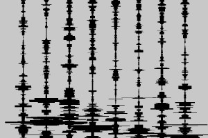
A couple days ago I read an article in the book about conserved economies. The idea is that you can model economic behavior if you make some simplifying assumptions (like that people spend exactly as much as they earn). What really intrigued me about the article were the graphs of wealth distribution over time. By slightly tweaking various economic parameters, it’s possible to make economies collapse by concentrating all wealth in the hands of one person.

I’ve been toying with Processing a lot lately, and these graphs finally gave me an excuse to get started. I wrote up a quick toy economy sketch and generated my own versions of the economies described in the book.

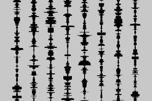
Wealth in a stable economy is rarely concentrated.

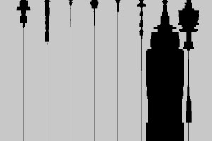
Wealth in an unstable economy all belongs to one person.

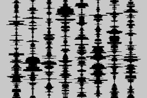
These economies are super simple. No one ever makes or loses money, except in a transaction with someone else. In those transactions, someone makes money and someone else loses money. Each line is a person’s wealth over time (time 0 is at the top). The width of the line corresponds to how much money they actually have.

So we’re basically assuming that everyone has some amount of money in savings, and that they spend exactly as much as they make. I like saving, so I added a savings feature. Everyone gets one unit of wealth each time step. In order to keep people from accumulating infinite wealth, I set up a random event that would force them to spend their savings. Now each person saves for a rainy day, and they periodically experience those rainy days and have to spend their savings.

Saving in a stable economy don\’t make a big difference.

Savings in an unstable economy aren\’t very realistic.

A normally stable economy remains essentially stable. People do manage to save up a higher maximum amount of money, but they don’t really keep it for very long. It also doesn’t give people a leg up in exchanges.

That changes in an unstable economy. The person who ends up owning all the wealth really gets it all. It’s kind of ridiculous. Surprisingly, even the people who don’t get very wealthy still don’t get as poor as they would have if they hadn’t saved a little. It seems that extra boost gives them a little more leverage in an exchange. One thing to keep in mind about this is that the agents aren’t allowed to go into debt. If agents could have negative money, this situation might be very different.

Since I’ve been interested in startups and entrepreneurs for a while, I decided to add that into my economy as well. I gave entrepreneurs some chance to win much more than they already have, but also to lose much of what they had. It turns out this is a hard thing to get stable. If succeeding in a startup is too hard (and too many people try), the entire economy collapses pretty quickly. On the other hand, if it’s very easy then everyone ends up ridiculously wealthy. It seems like that kind of situation would lead to hyperinflation, which wouldn’t really be a good thing.

Too many failed startup kill an economy.

A Goldilocks economy is just right. Everyone starts to get rich at the end.

Easy money means hyperinflation.

These models are way too simple to accurately represent a real economy. Real economies have a lot of intricacies that I didn’t want to go into for this. One of my EE professors once said that we’d never find the “Maxwell’s Equations of Economics” because there was simply too much going on. That’s probably true, but there’s something poetic about modeling economies in such a simple way.

Get the code here.

Counting eggs before they’re cooked

I eat a lot of eggs. Maybe three times a week, I’ll make myself an egg burrito for breakfast. I also tend to eat a lot of omelets for dinner. That’s six eggs a week for breakfasts, plus maybe four more for dinners. I eat a lot of eggs, which means I got through a lot of egg cartons.

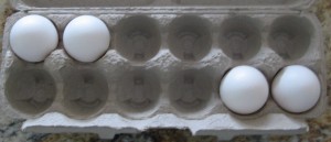
In the mornings, when I’m standing bleary eyed in front of the stove waiting for my eggs to cook, I often amuse myself by placing the remaining eggs into the carton in some symmetric fashion. I do this so often that I’ve started eating even numbers of eggs at a time, just to make sure I can put away the rest of the eggs symmetrically.

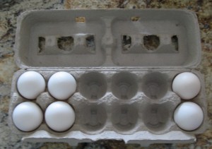
When I started doing this, I generally just tried to arrange them with symmetry about the x-axis. In this case, the x-axis divides a dozen egg carton in half hot-dog style (even though I eat lots of eggs, I don’t really buy the larger cartons). Arranging eggs in this manner is easy, because all you do is organize the bottom row in the same way as the top row.

Symmetry about the x-axis

Organizing eggs symmetrically got me thinking about how many ways I could actually pack them. For x-axis symmetry, I really only care about the top row. After I set the top row, the bottom row is uniquely defined. So if I have some even number of eggs, the number of ways I can put half of them into the top row is the same as the number of ways I can organize the eggs symmetrically.

It turns out that counting the number of ways I can put (for example) 2 eggs into 6 spots is given by the choose function. The choose function, (n choose k), is defined as the number of ways that you can pick k things from n possibilities. That’s exactly what I’m doing when I put eggs into a carton: I’m choosing 2 out of 6 possible places to put eggs.

This means that if I have 2n eggs left, for 0<=n<=6, there are (6 choose n) ways of organizing the eggs symmetrically. If I try every possibility each morning starting on the day that I got them (not on the day I first ate them) then I’ll have tried (6 choose 6) + (6 choose 5) + … = sum from i = 0 to 6 of (6 choose i).

Plugging this into Python, I get:

>>> from math import *
>>> sum = 0
>>> for i in range(7):
... sum += factorial(6)/(factorial(i)*factorial(6-i))
...
>>> sum
64

This is 64 possible combinations, just for vertical symmetry.

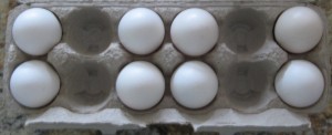
After a few months of eating eggs, I’d pretty much covered all of those. To make it a bit more interesting, I decided to go for horizontal symmetry instead. You still end up dividing the eggs and placing half of them in the left side of the carton. The right side is just a mirror of the first. At first, this seemed like it would be more interesting because instead of one row of eggs, I actually have three rows of two.

Symmetry about the y-axis

Unfortunately, the math works out exactly the same. There are still only six positions to place the eggs. This time the six are on one side, rather than on the top. While the positions might look slightly more interesting, there are the same number of them.

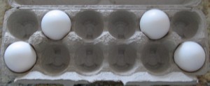
The last place to look for interesting symmetries in my dozen-egg carton is rotational. In this case, the carton would look the same if I rotated it 180 degrees. This only happens if the top right quadrant is the mirror of the bottom left. Same goes for top left and bottom right. So I’ve got my even number of eggs, and I can then divide them and put them however I want in the left quadrants, which defines the positions in the two right quadrants.

Symmetry about the origin

This is exactly the same as with both other forms of symmetry; the only change is how the new egg positions are defined.

The last thing that I’m interested in here is the combination of all three forms of symmetry. A carton packing that is symmetric about the x-axis and y-axis is also symmetric about the origin, but not all packings that are symmetric about the origin are also symmetric about both axes.

Symmetry about the x- and y-axes

To create symmetry about both axes, we only have choices in a single quadrant. Once one quadrant is packed, all three other quadrants are explicitly defined. This means that the total number of eggs has to be divisible by 4, not just 2. We can only do this with 12, 8, 4, and 0 eggs.

With 12 eggs and 0 eggs, there isn’t even a choice. Both those options give us a single method of creating symmetries. The 8 egg option means that there will be two eggs in each quadrant, for a total of (3 choose 2) symmetry options. The 4 egg option means that there’s one egg in each quadrant, giving us (3 choose 1) symmetry options.

(3 choose 2) = 3
and
(3 choose 1) = 3

This is because if you’re putting one object into three places, there are three possible ways to do it. If you’re putting two objects into three places, that’s the same as leaving one object out of three places. Thus the two are the same.

The total number of carton packings that are symmetric about both axes and the origin is then 1 + 1 + 3 + 3, or 8.

Now that I’ve actually worked out how many symmetries there are, I may get around to writing a program to generate them all. Sounds like I’m going to get more practice with Processing.

Arduino + Processing = Etch-a-Sketch

I’ve been using the Arduino for a few years now, but all of my projects with it were pretty self contained. I made some robots and some light controllers, but those things just sit there and do whatever it is they do. Until now, I’ve never used the Arduino as an analog front end for a PC. A lot of people seem to use the Arduino only for that purpose.

I was sitting around the other day thinking about this, and I decided I’d try to figure out how to do it. I could have just written something that would communicate with the Arduino over USB (kind of like RepG does with the MakerBot), but I only had an hour and I wanted to get something working quickly.

Enter Processing. I’ve only made one project with Processing before, but it did make it pretty easy. I’ve also heard that Processing interfaces with the Arduino easily. So now I had two tools, the Arduino and Processing, I just needed something to build with them. I looked in my junk box, and found two nice 100k potentiometers. This reminded me of the Propeller based Etch-A-Sketch. Since I didn’t have an Etch-a-Sketch handy, I just decided to use the potentiometers to draw pictures in Processing.

I hooked my Pots up to the first two analog inputs of my Arduino and did a quick google search. Turns out that processing communicates with a prewritten sketch called Firmata. The Arduino IDE comes with a couple of different versions of Firmata, each geared towards a different usage of the Arduino. The AnalogFirmata sketch worked pretty well for my needs.

A few minutes later, I’m twiddling my pots and drawing pictures. I also added a button to my sketch to allow me to save whatever I was drawing. This was actually the hardest part of the whole endeavor, because the AnalogFirmata didn’t have digital inputs. A little copy/paste action from the DigitalFirmata to the AnalogFirmata, and I was back in business.

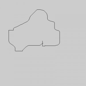
I drew Greenlake.

Etch-a-Sketch Greenlake
Ya, I never learned how to use a real etch-a-sketch either.

Find the Code here